Solving Fuzzy Linear Fractional Programming Problem using LU Decomposition Method

Vol. 13, No. 1, 2017, 89-97

ISSN: 2279-087X (P), 2279-0888(online) Published on 18 February 2017

www.researchmathsci.org

DOI: http://dx.doi.org/10.22457/apam.v13n1a9

89

Annals of

Solving Fuzzy Linear Fractional Programming Problem

using LU Decomposition Method

S.Muruganandam1 and P. Ambika2 1

Department of Mathematics, Imayam College of Engineering Tiruchirappalli-621 206, Tamil Nadu, India. Email: [email protected]

2

Department of Mathematics, M.A.M. College of Engineering & Technology Tiruchirappalli-621 105, Tamil Nadu, India. Email: [email protected]

Received 17 January 2017; accepted 15 February 2017

Abstract. This paper proposes a new approach to solve fuzzy linear fractional programming problem (FLFPP). In this paper, the FLFPP is converted into crisp linear fractional programming problem (LFPP) using ranking method. The converted LFPP is then solved by LU Decomposition method. An illustrated example shows the simplicity of the proposed approach.

Keywords: Linear fractional programming, LU decomposition, triangular fuzzy number. AMS Mathematics Subject Classification (2010): 90C32, 03E72

1. Introduction

Linear fractional programming problem is mainly used in decision making process in which the objective function is a fraction of two linear functions. Fractional programming problems are used in many fields such as production planning, financial and corporate planning, health care and hospital planning, etc. Many researchers found various techniques to solve linear fractional programming problems.

90

projection method for solving LFPP. LU Decomposition is just a compact and relatively numerically stable method to solve a system of linear equations. For large n, the

computational time for LU Decomposition is proportional to , while for Gaussian

Elimination, the computational time is proportional to . So for large n, the ratio of the computational time for Gaussian elimination to computational time for LU

Decomposition is . As an example, for the coefficient matrix of order 2000×2000, computational time by Gaussian Elimination would take n/4=2000/4=500 times the time it would take for LU Decomposition.

This paper is outlined as follows. Section 2 gives the preliminaries of the fuzzy number. In Section 3, mathematical formulation of the FLFPP is given. Section 4 describes the proposed method and Section 5 explains how the proposed method is applied to the LFPP. In Section 6, Yager’s ranking method [10] is given and Section 7 gives the illustrated example and Section 8 concludes the paper.

2. Preliminaries

In this section, some basic definitions relating to fuzzy sets and triangular fuzzy numbers are given.

Definition 2.1. A fuzzy set A is called normal if there is at least one element such

that .

Definition 2.2. A fuzzy set A is called convex if for any and any ,

.

Definition 2.3. The

α

Definition 2.4. A fuzzy set is a fuzzy number if it satisfies the conditions of normality and convexity.

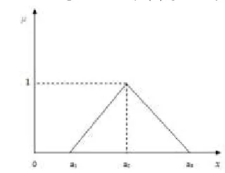
Definition 2.5. Triangular fuzzy number

A triangular fuzzy number with membership function given by

X

x

∈

( )

A

µ

X y

x, ∈

λ

[ ]

(

)

(

x

y

)

{

( ) ( )

x

y

}

A

λ

λ

µ

µ

µ

+

1

−

≥

min

,

( )

{

µ

α

}

α

=

x

∈

X

x

≥

A

/

)

,

,

(

~

3 2 1

a

a

a

a

=

µ

( )

x

  

   

 

≤ ≤ −

−

≤ ≤ −

−

=

elsewhere a x a for a a

x a

a x a for a a

a x

x

, 0

, ,

)

( 2 3

2 3

3

2 1

1 2

1

µ

Method

91 Mathematical Formulation of FLFPP

Maximize

Subject to

where is an n-dimensional vector of decision variables, and are vectors,

is an constraint fuzzy matrix, is an - dimensional fuzzy vector, and are scalars.

3. LU decomposition method

Given a system of ‘ ’ linear equations with unknowns. We write this system as

where ,

(i) Write , where L is the unit lower triangular matrix and U is the upper triangular matrix. From this equation, we find L and U.

(ii) Now the system of equations becomes . (iii) Let . Now, we solve for

(iv) Using , we solve for . This will give the solution for the system .

4. Application of LU decomposition method to solve linear fractional programming problem

Consider the following Linear Fractional Programming Problem.

……… (1)

Let us convert this linear fractional programming problem into linear programming problem using Charnes and Cooper method as below.

β

α

~ ~

~ ~ ~

+ + =

x d

x c

z _T

T

0 ~ ~

≥ ≤

x b x A

x

c

~

,

d

~

n

m× b~ m α~ β~

n n

B

AY =

[ ]

n n ij

a

A= _×

[ ]

1 ×

= y_{j n}

Y B=

[ ]

LU A=

B

LUY =

W

UY = LW = B W

W UY =W Y

B AY =

0 ,...,

,

....

... ... ... ... ... ...

.... ... ... ... ... ...

.... ....

... ...

2 2

1

2 2 , 2

2 1 1

4 2 2 , 4 2

42 1 41

3 2 2 , 3 2

32 1 31

2 2 2

2 1 1

2 2 2

2 1 1

≥

≤ +

+ +

≤ +

+ +

≤ +

+ +

+ +

+ +

+ +

+ + =

−

− −

− −

− −

− −

− −

n

n n n n n

n

n n

n n

n n

n n

x x

x

b x a x

a x a

b x a x

a x a

b x a x

a x a

to Subject

x d x

d x d

x c x

c x c z Maximize

92

Let and for

Now, we write the problem (1) as the following LPP.

,,, ,,, ,,, (2)

We write this LPP in the form of less than or equality constraints.

……… (3)

Now the system of equations can be considered as where

β + + + + = − −2 2 2 2 1 1 ... 1 n n x d x d x d

t yi =txi, i=1,2,3...,n−2

Method

93 .

Yager’s ranking method

Given a convex triangular fuzzy number , the -cut of the fuzzy number is given by

The Yager’s Ranking index [10] is defined by

,

where is a -level cut of fuzzy number .

5. Numerical example Consider the following FLFPP

Subject to

ሺ1,5,9ሻݔ_ଵ+ ሺ2,3,4ሻݔ_ଶ≤ ሺ5,6,7ሻ

ሺ4,5,10ሻݔ_ଵ+ ሺ0,1,2ሻݔଶ≤ ሺ4,6,8ሻ ……… (4)

ݔଵ, ݔଶ≥ 0

Now, we convert the FLFPP into the following crisp LFPP using Yager’s ranking method.

The -cut of fuzzy number is

Proceeding similarly, the problem (4) can be written as the following crisp LFPP

Subject to        

 

       

 

=

−

z t y

y y

Y

n 2

2 1

...

       

 

       

 

=

0 ... 0 0 1 0

B

(

)

C~= , ,

α

C~

(

)

(

(

)

α

(

)

α

)

( )

(

)

α

R =

∫

1 0

5 . 0 ~

(

)

C

C_α + _α

α

(

)

(

)

(

)

( )

(

)

2 , 1 , 0 3 , 2 , 1

2 1

2 1

+ +

+ =

x x

x x

z Maximize

α

(

)

(

)

(

α

α

)

(

)

(

)

1 0

= −

+ +

=

_∫

α

α

α

R

6 3

2

2 1

2 1

+ +

+ =

x x

x x z

94

Let and

The given LFPP becomes a LPP as below.

Subject to

Solution by LU decomposition method:

We write the above LPP as

We write the system as

where , , .

We write where L is a unit lower triangular matrix U is an upper triangular matrix.

t x

x + +6 =

3 1

2 1

2 2 1

1 y ,tx y

tx = =

2 1

2y y z

Maximize = +

0 , ,

0 6 3 5

0 6 7

1 6 3

2 1

2 1

2 1

2 1

≥ ≤ − +

≤ − +

= + +

t y y

t y y

t y y

t y y

0 , ,

0 6 3 5

0 6 7

1 6 3

0 2

2 1

2 1

2 1

2 1

2 1

≤ − − −

≤ − +

≤ − +

= + +

≤ + − −

t y y

t y y

t y y

t y y

z y y

B AY =

   

 

   

 

− − − −

=

0 6 3 5

0 6 1 7

0 6 1 3

1 0 1 2

A

   

 

   

 

=

z t y y

Y 2

1

   

 

   

 

=

0 0 1 0

B

LU A= 0 ,

6 7

6 3 5

2 1

2 1

2 1

≥ ≤ +

≤ +

x x

x x

Method

95

That is, and

Now,

On simplification, we get,

Thus, ,

Now, . We write where .

Now, we solve LW=B for W, where             = 1 0 1 0 0 1 0 0 0 1 43 42 41 32 31 21 l l l l l l L             = 44 34 33 24 23 22 14 13 12 11 0 0 0 0 0 0 u u u u u u u u u u U             − − − − =                         0 6 1 3 0 6 1 7 0 6 3 5 1 0 1 2 0 0 0 0 0 0 1 0 1 0 0 1 0 0 0 1 44 34 33 24 23 22 14 13 12 11 43 42 41 32 31 21 u u u u u u u u u u l l l l l l 4 , 0 , 1 , 2 5 , 4 , 36 , 5 , 2 7 , 2 3 , 6 , 2 1 , 2 3 , 1 , 0 , 1 , 2 44 43 42 41 34 33 32 31 24 23 22 21 14 13 12 11 = = − = − = − = − = − = − = = = − = − = = = − = − = u l l l u u l l u u u l u u u u                   − − − − = 1 0 1 2 5 0 1 5 2 7 0 0 1 2 3 0 0 0 1 L               − − − − − = 4 0 0 0 4 36 0 0 2 3 6 2 1 0 1 0 1 2 U B

LUY = LW =B UY =W

96 On simplification, we get

Finally, the solution matrix is given by UY=W.

That is,

On simplification we get,

Thus, the optimal solution of the LFPP is given by

6. Conclusion

In this paper, we proposed a new approach called LU Decomposition Method of matrices to solve fuzzy linear fractional programming problem (FLFPP). The FLFPP is converted into crisp LFPP using Yager’s Ranking method and then it is converted into LPP using Charnes and Cooper method. In this approach, we get the solution directly and the time consumption is very less. A numerical example is given to show the simplicity of the proposed approach and the solution is verified by LINGO 13.0 version also.

Acknowledgement. The authors thank the anonymous referees and the Chief-Editor for their valuable comments and suggestions, which were very helpful in improving the presentation of this paper.

   

 

   

 

=

   

 

   

 

      

 

      

 

− − − −

0 0 1 0

1 0 1 2 5

0 1 5 2 7

0 0 1 2 3

0 0 0 1

4 3 2 1

w w w w

   

 

   

 

=

z t y y

Y 2

1

   

 

   

 

− =

   

 

   

 

    

 

    

 

− − −

− −

1 5 1 0

4 0 0 0

4 36 0

0 2

3 6 2 1 0

1 0 1 2

2 1

z t y y

4 1 , 9 1 , 12

1 ,

12 1

2

1 = y = t = z= y

4 1 , 4 3 ,

4

3 ₂

2 1

1 = = = = z= t

y x t

y x

1 , 5 ,

1 ,

0 _{2 3 4}

Method

97 REFERENCES

1. A.Charnes and W.W.Cooper, Programs with linear fractional functions, Naval Research Logistics Quarterly, 9 (1962) 181-196.

2. S.M.Chinchole and A.P.Bhadane, LU factorization method to solve linear programming problem, Intern. J. Emerging Technology and Advanced Engineering, 4(4) (2014) 176-180.

3. N.Jayanth Karthik and E.Chandrasekaran, Solving fully fuzzy linear systems with trapezoidal fuzzy number matrices by partitioning the block matrices, Annals of Pure and Applied Mathematics, 8(2) (2014) 261-267.

4. P.Pandian and K.Kavitha, A new method for solving fuzzy assignment problems, Annals of Pure and Applied Mathematics, 1(1) (2012) 69-83.

5. S. Radhakrishnan, P. Gajivaradhan and R. Govindarajan, A new and simple method of solving fully fuzzy linear system, Annals of Pure and Applied Mathematics, 8(2) (2014) 193-199.

6. S.Jain, Modified gauss elimination technique for separable nonlinear programming problem, International Journal of Industrial Mathematics, 4(3) (2012) 163-170. 7. S.C.Sharma and A.Bansal, An integer solution of fractional programming problem,

Gen. Math. Notes, 4 (2001) 1-9.

8. K.Swarup, Linear fractional functional programming, Operation Research, 13 (1965) 1029-1036.

9. S.F.Tantawy, A new procedure for solving linear fractional programming problems, Mathematical and Computer Modelling, 48 (2008) 969-973.