ISSN: 2321 – 9238 (online) Published on 3 June 2013 www.researchmathsci.org
39
ABC Optimization: A Co-Operative Learning Approach
to Complex Routing Problems
P.K. Saranya and K. Sumangala Department of Computer Science
Vellalar College for Women Erode – 638 012, Tamil Nadu, India
Email: [email protected], [email protected]
Received 15 May 2013; accepted 31 May 2013
Abstract. Many practical and complex problems in industry and business such as the routing problems, scheduling, networks design, telephone routing etc.,. are in the class of intractable combinatorial (discrete) or numerical (continuous or mixed) optimization problems. Many traditional methods were developed for solving continuous optimization problems, while discrete problems are being solved using heuristics. In the past few years, several modern metaheuristic algorithms that apply to both domains have been developed for solving such problems .They include population based, iterative based, stochastic, deterministic and other approaches. Classification can be made in two important groups of natural inspired and population based algorithms: evolutionary algorithms (EA) and swarm algorithms.
The proposed method has been developed to detect and extract the best availability shortest traversal path for any complex routing problems. It uses an efficient Artificial Bee Colony algorithm based on the foraging behaviour of honey bees for solving numerical optimization problems.
Keywords: Ant-colony optimization (ACO), Continuous Ant Colony optimization (CACO), MAX –MIN Ant System (MMAS),
Artificial Bee Colony algorithm
(ABC)
, Swarm Intelligence (SI).1. Introduction
40
substance known as pheromone along the way between their colony and food source. Bees perform waggle dance upon returning to their hive when they found a food source. Pheromone trail and waggle dance are used as a communication medium among individuals in ant or bee colony. These individuals usually perform their actions (depositing pheromone or performing waggle dance) locally with limited knowledge about the entire system. However, when their local actions are combined, they will emerge to produce global effects such as directing more individuals to the new discovery of food source. We already described about Ant Colony Optimization (ACO) and Continuous ACO with MMAS algorithm for TSP in [3]. Our initial work showed that the original ABC algorithm to TSP could be improved further. The proposed model is based on bee foraging behaviour where bees are used to generate feasible solutions for TSP benchmark problems found in TSPLIB1 through the integration of ABC algorithm. This paper undergoes five phases of operation to accomplish the resultant shortest traversal path. Finally, this paper ends with conclusion and future works.
2. Traveling Salesman Problem (TSP)
The Travelling Salesman Problem (TSP) is an NP-hard problem in combinatorial optimization studied in operations research and theoretical computer science. Given a list of cities and their pair wise distances, the task is to find a shortest possible tour that visits each city exactly once. The problem was first formulated as a mathematical problem in 1930 and is one of the most intensively studied problems in optimization.The TSP is a very important problem in the context of Ant Colony Optimization because it is the problem to which the original AS was first applied, and it has later often been used as a benchmark to test a new idea and algorithmic variants.
The TSP was chosen for many reasons:
• It is a problem to which the ant colony metaphor
• It is one of the most studied NP-hard problems in the combinatorial optimization • It is very easily to explain. So that the algorithm behavior is not obscured by too
many technicalities.
41 3. Artificial Bee Colony Algorithm
Karaboga (2005) analyzes the foraging behaviour of honey bee swarm and proposes a new algorithm simulating this behaviour for solving multi-dimensional and multi-modal optimization problems, called Artificial Bee Colony (ABC). The artificial bee colony algorithm is a new population-based metaheuristic approach. It has been used in various complex problems. The algorithm simulates the intelligent foraging behavior of honey bee swarms. The algorithm is very simple and robust. In the ABC algorithm, the colony of artificial bees is classified into three categories: employed bees, onlookers, and scouts.
The steps involved in the proposed algorithm are :
Step 1: Initializing the population: First fit the range (area), lower boundary area and colony by inputting the upper bound (ub), lower bound (lb), colony size and its dimensionality. Range is the difference between the highest and the lowest values in a frequency distribution. Therefore the range of matrix is calculated by the function Repmat(A, m, n) where it creates a large matrix by tiling of A with m copies of A in the row direction, and n copies of A in the column direction.
Figure 1:
Range = repmat( (ub – lb), [colonysize colonydimension])
42
Colony = rand (colonysize , colonydimension) * range + lower
The employed bees are initialized by specifying the one half of the colony area. Here the lower bound is the nest or the sources were the bees start its process. The colony area is the area we specified for solving traversal problem.
Step 2: Selection Strategy of Artificial Bee Colony Algorithm a) Evaluating the fitness:
In the exploitation process of onlooker bees in ABC algorithm, onlooker bees choose food source by a stochastic selection scheme. The selection strategy consists of three steps: first, calculating fitness value; second, calculating selection probability for each solution in population; third, selecting candidate solution according to selection probability by “roulette wheel selection” method, and then starting neighborhood search. Fitness function is considered as evidence to distinguish the good or bad individuals. Selection a good fitness function is very important which can keep population diversity and avoid premature convergence. Fitness function F(x) is usually a mathematical transformation from objective function f(x).
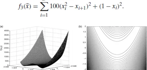
The objective function f(x) is calculated by the Benchmark function. The search process must be able to avoid the regions around local minima in order to approximate, as far as possible, to the global optimum. The most complex case appears when the local optima are randomly distributed in the search space. The dimensionality of the search space is another important factor in the complexity of the problem. The five classical benchmark functions are Griewank function, Rastrigin function, Rosenbrock function, Ackley function and Schwefel function. In this work f(x) is calculated by the Rosenbrock
function .
Rosenbrock function whose value is 0 at its global minimum (1,1,…,1) using following equation. Initialization range for the function is [−15, 15]. The global optimum is inside a long, narrow, parabolic shaped flat valley. Since it is difficult to converge the global optimum, the variables are strongly dependent, and the gradients generally do not point towards the optimum, this problem is repeatedly used to test the performance of the optimization algorithms. x is in the interval of [-50, 50]. Global minimum value for this function is 0 and optimum solution is xopt =(x1, x2, . . . , xn) = (1, 1, . . . , 1). Global optimum is the only optimum, function is unimodal. Surface plot and contour lines of
f(x) are shown in Figure 2 and the function is calculated by the formula given below
43
Initialize the cycle value by 1. Perform the below process until the condition cycle met.
Step 3: Searching neighborhood (new food source) Employed phase:
Employed bees search for new food sources (vij) having more nectar within the
neighbourhood of the food source (xij) in their memory. They find a neighbour food
source and then evaluate its profitability (fitness). For example, they can determine a neighbour food source vij using the formula given by equation below.
vij = xij +
φ
ij ( xij - xkj)where k =1, 2, …, NS and j ={1, 2, …, D} are randomly chosen indexes. It must be noted that k has to be different from i.
φ
ij is a random number between [-1, 1]. Parameter values produced by the above equation which exceed their boundary values are set to their boundary values. It searches all the nodes and each Bee finds their shortest covering distance node.Step 4: Memorize the best source
After generating the new food source, the nectar amount of it will be evaluated and a greedy selection will be performed. If the quality of the new food source is better than the current position, the employed bee leaves its position and moves to the new food source; in other words, If the fitness of the new food source is equal or better than that of Xi, the new food source takes the place of Xi in the population and becomes a new member.
Step 5: Selecting best food source Onlooker phase:
First an onlooker bee selects a food source by evaluating the information received from all of the employed bees. The probability pi of selecting the food source i is determined by:
where fi is the fitness value of the food source Xi. After selecting a food source, the onlooker generates a new food source using the above equation. Once the new food source is generated, it will be evaluated and a greedy selection will be applied, same as the case of employed bees.
Step 6: Scout phase - accepting or abandoning the new food
44
vij = xmin j + rand [0, 1] x ( xmax j – xmin j ) for j = 1, 2,…, D.
The abandoned food source is replaced by the randomly generated food source. In the ABC algorithm, the predetermined number of trials for abandoning a food source is called limit, also in this algorithm at most one employed bee at each cycle can become a scout.
Step 7: Increasing the cycle value
If a termination condition is met, the process is stopped and the best food source is reported; otherwise the algorithm returns to step 3.
4. Results and Discussions
To demonstrate our proposed algorithm ABC experimentally and compare its performance with ACO and CACO with MMAS, we have created a simulation environment. This environment is called Beehive that is virtually illustrated .Our comparison is based on efficiency, scalability and adaptability. In this work, two classification problems are considered in which one is taken from repository of UCI data repository (Frank and Asuncion, 2010) are used to evaluate the performance of Ant Colony Optimization and Artificial Bee Colony Algorithm. The selected problems are Travelling Salesperson (TSP) datasets whose file names are located on TSPLIB. Another one is taken from North American Numbering Plan, telephone routing. The telephone routing dataset is recorded on April 1999, which include the area code and exchanges registered for use in the USA and Canada.
5. Experimental Setup
In order to evaluate the performance of the proposed algorithm, three datasets from TSPLIB and one from NANP – telephone routing are taken. They include “ npdata1.tsp”, “pr76.tsp”, “ch150.tsp” and “npanxx99.txt”.
The ‘inpdata1.tsp’ includes 22 cities problem Odyssey of Ulysses (Groetschel/Padberg) with dimension of 22 and find the edge detection using Geometric distance equation.
The ‘pr76.tsp’ includes 76 cities problem (Padberg/Rinaldi) with dimension of 76 and find the edge weight detection using the Euclidean distance.
The ‘ch150.tsp’ includes 150 cities problem (churritz) with dimension of 150 and find edge detection using the Euclidean distance.
The TSP dataset includes the parameters such as node, coordinates and the section.
Dataset Algorithm Dimension (nodes)
Mean (Error rate)
Standard Deviation
inpdata1.tsp
ACO 22 2.355272 1.769675
CACO 22 1.331720 1.301473
ABC 22 0.440508 0.363889
pr76.tsp ACO 76 2.906279 1.963521
45
ABC 76 0.460159 0.289092
ch150.tsp
ACO 150 3.285141 2.138416
CACO 150 2.093640 1.698724
ABC 150 0.488307 0.311342
Table 1: Comparison of algorithms
The mean and the standard deviations of the function values obtained by ABC, and ACO and CACO with MMAS for TSP files are given in the above Table.
The telephone routing dataset such as ‘npanxx99.txt’ contains 105291 NPA/NXX's (area code plus exchanges) registered for use in the USA and Canada.
It includes the parameter such as node as area and its distance to other nodes as exchanges.
The mean and the standard deviations of the function values obtained by ABC, and ACO and CACO with MMAS for Telephone Routing file are given in Table 1.
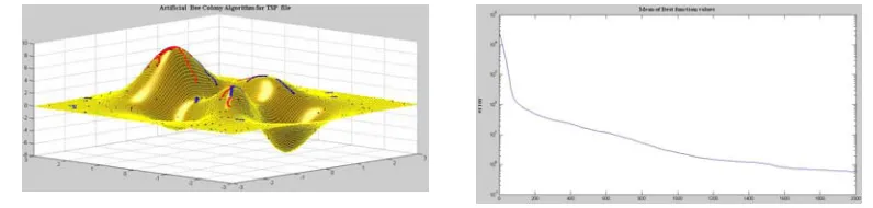
Sample screen:
Figure 3: Result of ABC algorithm for travelling salesperson : “inpdata1.tsp”
As seen from the above results, it shows that the ABC algorithm can converge to the minimum of Rosenbrock function, too. In other words, this proves that the ABC algorithm has the ability of getting out of a local minimum in the search space and finding the global minimum. In the ABC algorithm, while the exploration process carried out by artificial scouts is good for global optimization, the exploitation process managed by artificial onlookers and employed bees is very efficient for local optimization.
6. Conclusion
In this work, Artificial Bee Colony algorithm which is a recently introduced optimization algorithm is used to solve routing dataset which are widely used benchmark problems. To focus the performance of the ABC algorithm, ACO , CACO with MMAS and ABC algorithms were tested on high dimensional numerical benchmark functions that have multimodality.
46
local and global search which takes these solutions to a local and global optimum seems to be the best strategy.
From the simulation results it was concluded that the proposed algorithm has the ability to get out of a local minimum and can be efficiently used for multivariable, multimodal function optimization. Thus the system has shown that ABC is also a very good constructive heuristic to provide such starting solutions for both local and global optimizers. ABC with benchmark function-Rosenbrock gives less error rate and deviation from actual search compare with existing ACO, CACO with MMAS.
7. Further Research
The work can be extended further to other probabilistic optimization problems such as medical disease diagnosis and operation research problems.
In addition to Artificial Bee Colony algorithm, further study can be combined and analyzed using other metaheuristic algorithms like fuzzy, neural network and genetic algorithms to solve vast range of real life problems.
REFERENCES
1. K. von Frisch, Decoding the language of the bee, Science, 185 (4152) (1974) 663-668.
2. M. Dorigo and T. Stützle, The ant colony optimization metaheuristic: algorithms, applications, and advances, in Handbook of Metaheuristics, Springer, New York, 57 (2002) 250-285.
3. K.Sumangala and P.K.Saranya, Max-Min Ant system for Continuous ACO (CACO) for TSP,
International Journal of Advanced Computational methods and
Applications(
IJACA), 1(1) (2011) 13.4. D. Karaboga, An idea based on honey bee swarm for numerical optimization, Technical Report TR06, Computer Engineering Department, Erciyes University, Turkey, 2005.
5. D. Karaboga and C. Ozturk, A novel clustering approach: artificial bee colony algorithm, to appear in Applied Soft Computing.
6. R. S. Parpinelli, H. S. Lopes, and A. A. Freitas, Data mining with an ant colony optimization algorithm, IEEE Trans. Evol. Comput., 6(4) (2002) 321–332.
7. D. Parrott and X. Li, Locating and tracking multiple dynamic optima by a particle swarm model using speciation, IEEE Trans. Evol. Comput., 10(4) (2006) 440–458. 8. P.-W.T.Sai, J.-S. Pan, B.-Y. Liao and S.-C. Chu, Enhanced Artificial Bee Colony
Optimization, International Journal of Innovative Computing, Information and Control, 5(12) (2009) 1-ISII08-247.
9. V. Tereshko, Reaction-diffusion model of a honeybee colony’s foraging behavior, In: Schoenauer M. (ed.) Parallel Problem Solving from Nature VI. Lecture Notes in
Computer Science, 1917 (2000) 807–816, Springer, Berlin.