River temperature behaviour in changing environments: trends, patterns at different spatial and temporal scales and role as a stressor

(1)

Erasmus Mundus Joint Doctorate School in Science for MAnagement of Rivers and their Tidal System

Roshni Arora

River temperature behaviour in changing

environments: trends, patterns at different spatial and

temporal scales and role as a stressor

(2)

(3)

This thesis work was conducted during the period 1st October 2012 - 15th December 2015, under the supervision of Dr. Markus Venohr (Leibniz Institute of Freshwater Ecology and Inland Fisheries Berlin), Dr. Martin T. Pusch (Leibniz Institute of Freshwater Ecology and Inland Fisheries Berlin), Dr. Marco Toffolon (University of Trento, Italy) and Dr. Klement Tockner (Freie Universität Berlin) at Freie Universität Berlin, University of Trento, Italy and Leibniz Institute of Freshwater Ecology and Inland Fisheries Berlin.

1st Reviewer: Prof. Dr. Klement Tockner 2nd Reviewer: Prof. Dr. Gunnar Nützmann

(4)

(5)

The SMART Joint Doctorate Programme

Research for this thesis was conducted with the support of the Erasmus Mundus Programme1, within the framework of the Erasmus Mundus Joint Doctorate (EMJD) SMART (Science for MAnagement of Rivers and their Tidal systems). EMJDs aim to foster cooperation between higher education institutions and academic staff in Europe and third countries with a view to creating centres of excellence and providing a highly skilled 21st century workforce enabled to lead social, cultural and economic developments. All EMJDs involve mandatory mobility between the universities in the consortia and lead to the award of recognised joint, double or multiple degrees.

The SMART programme represents a collaboration among the University of Trento, Queen Mary University of London, and Freie Universität Berlin. Each doctoral candidate within the SMART programme has conformed to the following during their 3 years of study:

(i) Supervision by a minimum of two supervisors in two institutions (their primary and secondary institutions).

(ii) Study for a minimum period of 6 months at their secondary institution

(iii) Successful completion of a minimum of 30 ECTS of taught courses

(iv) Collaboration with an associate partner to develop a particular component / application of their research that is of mutual interest.

(v) Submission of a thesis within 3 years of commencing the programme.

1_{This project has been funded with support from the European Commission. This}

(6)

(7)

I

Summary

River/stream water temperature is one of the master water quality parameters as it controls several key biogeochemical, physical and ecological processes and river ecosystem functioning. Thermal regimes of several rivers have been substantially altered by climate change and other anthropogenic impacts resulting in deleterious impacts on river health. Given its importance, several studies have been conducted to understand the key processes defining water temperature, its controls and drivers of change. Temporal and spatial river temperature changes are a result of complex interactions between climate, hydrology and landscape/basin properties, making it difficult to identify and quantify the effect of individual controls. There is a need to further improve our understanding of the causes of spatiotemporal heterogeneity in river temperatures and the governing processes altering river temperatures. Furthermore, to assess the impacts of changing river temperatures on the river ecosystem, it is crucial to better understand the responses of freshwater biota to simultaneously acting stressors such as changing river temperatures, hydrology and river quality aspects (e.g. dissolved oxygen levels). So far, only a handful of studies have explored the impacts of multiple stressors, including changing river temperature, on river biota and, thus, are not well known.

(11)

Summary

V

be the major control of increasing river temperatures and of its temporal variability, with increasing influence for increasing catchment area and lower altitudes (lowland rivers). Strongest river temperature increase was observed in areas with low water availability. Other hydro-climatological variables such as flow, baseflow, NAO, had significant contributions in river temperature variability. Spatial variability in river temperature trend rates was mainly governed by ecoregion, altitude and catchment area via affecting the sensitivity of river temperature to its local climate. At a reach scale as well, air temperature was the major control of the temporal variability in river temperature over a period of nine months within a 200 km lowland river reach. The spatial heterogeneity of river temperature in this reach was most apparent during warm months and was mainly a result of the local landscape settings namely, urban areas and lakes. The influence of urban areas was independent of its distance from the river edge, at least when present within 1 km. Heat advected from upstream reaches determined the base river temperature while climatological controls induced river temperature variations around that base temperature, especially below lakes. Riparian buffers were not found to be effective in substantially moderating river temperature in reaches affected by lake warming due to the dominant advected heat from the upstream lake. Experimental investigation indicated that increasing water temperature had a stronger short-term effect on behavioural responses of benthic invertebrates, than simultaneous changes in flow or dissolved oxygen. Also, increases in water temperature was shown to affect benthic invertebrates more severely if accompanied by concomitant low dissolved oxygen and flow levels, while interactive effects among variables vary much among taxa.

(12)

Summary

VI

(13)

Zusammenfassung

VII

Zusammenfassung

Die Wassertemperatur ist ein zentraler Wasserqualitätsparameter, der eine Vielzahl verschiedener biogeochemischer, physischer und ökologischer Prozesse sowie Ökosystemfunktionen von Flüssen steuert. Das Temperaturregime vieler Flüsse wurde bereits nachhaltig durch Klimawandel und andere anthropogene Einflüsse verändert und beeinflusst den chemischen und ökologischen Zustand der Flüsse. Angesichts dieser Bedeutung, haben bereits mehrere Studien die beteiligten Prozesse, Steuergrößen und anthropogenen Überprägungen der Wassertemperatur untersucht. Zeitliche und räumliche Temperaturänderungen resultieren aus einer komplexen Wechselwirkung zwischen Klima, Hydrologie und Einzugsgebietseigenschaften. Die Identifikation und Quantifizierung der Effekte einzelner Steuergrößen ist dementsprechend schwierig. Trotz früherer Studien besteht ein weiterer Forschungsbedarf um die Ursachen der raum-zeitlichen Heterogenität von Wassertemperaturen und ihrer maßgebenden Steuerungsprozesse vollständig zu verstehen. Darüber hinaus ist es entscheidend die Reaktionen von Süßwasserorganismen auf gleichzeitig wirkende Stressoren wie veränderte Wassertemperatur, Hydrologie und Wasserqualitätsaspekte (z.B. Gehalt an gelöstem Sauerstoff) besser zu verstehen um die Bedeutung von Temperaturregimeänderungen vollständig erfassen zu können. Bisher haben nur wenige Studien die Auswirkungen multipler Stressoren, einschließlich der Änderung der Wassertemperatur, auf Süßwasserorganismen untersucht.

(14)

Zusammenfassung

VIII

Wassertemperatur, Strömung und dem Gehalt von gelöstem Sauerstoffs experimentell untersucht.

(15)

Zusammenfassung

IX

(16)

Zusammenfassung

(17)

XI

Thesis outline

This thesis is composed of three manuscripts that are either accepted for publication, or ready to be submitted to peer-reviewed journals. Each manuscript has an introduction, methodology, results and discussion and forms a chapter of the thesis. A general introduction section provides the general context of the thesis and the results are discussed coherently a s the general discussion section. The layout of the three manuscripts was modified and figures and tables were renumbered through the text to ensure a consistent layout throughout the entire thesis. The references of the general introduction, each manuscript, and general discussion were merged in an overall reference section. The research aims of Chapters 2, 3 and 4 are described in Paragraph 1.4.

Chapter 1:

General introduction Chapter 2:

Arora R, Tockner K, Venohr M. (submitted to Hydrological Processes). Changing river temperatures in Northern Germany: trends and drivers of change.

Author Contributions:

R. Arora designed the study, analysed the data and compiled the manuscript. K. Tockner and M. Venohr co-designed the study and contributed to the text. Chapter 3:

Arora R, Toffolon M, Tockner K, Venohr M. (to be submitted) Influence of landscape variables in inducing reach-scale thermal heterogeneity in a lowland river.

(18)

co-XII

designed the study and contributed to the text. K. Tockner co-designed the study.

Chapter 4:

Arora R, Pusch MT, Venohr M. (to be submitted) Interactions between effects of experimentally altered water temperature, flow and dissolved oxygen levels on aquatic invertebrates.

R. Arora designed the study, organized and performed field and laboratory work, analysed the data and compiled the manuscript. M.T. Pusch co-designed the study and contributed to the text. M. Venohr co-co-designed the study.

Chapter 5:

(19)

(20)

XIV

List of Tables

Table II.1 Recent studies on river temperature trends worldwide (updated

from Kaushal et al., 2010) ………15

(21)

XV

(22)

(23)

XVII

List of Figures

(24)

XVIII

Figure SII.2 Cumulative frequency distribution (ecdf) for proportion of forest, agriculture and urban land use cover types within 1 km2 site buffers (time period:2000-2010; n=112)………...127 Figure SII.3 Cumulative frequency distribution of significant air temperature (AT)-river temperature (RT) slopes from linear regression for both time periods………..128 Figure SII.4 Frequency of months with mean monthly river temperature above the threshold temperature of 22°C plotted for several sites. The threshold temperature was based on thermal limits of fish and invertebrate species as mentioned in Hardewig et al. (2004), Haidekker & Hering (2008) and Vornanen et al. (2014)………...………...129 Figure III.1 Maps showing the location of the study area, stream temperature (ST) measuring locations, and the thermally heterogeneous sub-reaches. Stream temperature measuring locations are numbered corresponding to their IDs (Table 3.2)……….…………..43 Figure III.2 Daily means for the 4th (blue), 10th (dark green) and 15th (black) day of each month plotted for the 20 sites on River Spree for all months during the study period………..…55 Figure III.3 Boxplots showing 𝐸𝑟 values for the entire study period (a), for

(25)

XIX

daily mean hydroclimatological variables and ST for all sites on River Spree………..61 Figure III.6 Root Mean Square Errors (RMSE) for the three models for all sites on River Spree………..………...68 Figure III.7 Spatial variation of the air2stream parameters. Plots show the ratios of the main model parameters to 𝑐₃ (𝐶₁, 𝐶₂, 𝐶₃, 𝐶₄; see equation 8)...58 Fig. SIII.1 Share of cover of different land use types within 50, 100, 500 and 1000 m buffer widths at all sites on River Spree………..………...…133 Fig. SIII.2 Daily range (maximum-minimum) for the 15th day of each month plotted for 20 sites on River Spree for all months…………...…………....134 Fig. SIII.3 Plots showing the nature of relationship of ST with different atmospheric variables. The curves were determined by the non-linear models using the spline-smoothing function (function gam in mgcv package, R)..135 Figure IV.1 Sketch of the experimental flume………..…….…84 Figure IV.2 Interaction plot of flow and DO for the three study species showing the mean number of detached individuals (average for the three replicates ± SE, n=10 for D. haemobaphes and H.pellucidula; n=9 for C.

splendens)………....…..87

Figure IV.3 Interaction plot of water temperature and DO for the three study species showing the mean number of detached individuals (average for the three replicates ± SE, n=10 for D. haemobaphes and H.pellucidula; n=9 for

C. splendens)……….….89

Figure IV.4 Interaction plot of water temperature and flow for the three study species showing the mean number of detached individuals (average for the three replicates ± SE, n=10 for D. haemobaphes and H.pellucidula; n=9 for

C. splendens)………..91

(26)

XX

(27)

(28)

Chapter 1 General introduction

1

1. General introduction

1.1 River temperature: importance in ecosystem functioning and research history

Rivers are hierarchical systems (Montgomery, 1999) in which physical variables such as water temperature, channel area, velocity, flow volume, are present in a continuous gradient of conditions (river continuum concept, Vannote et al., 1980). Among these various variables, river temperature is a physical property of prime importance as it controls physicochemical and ecological processes within freshwater ecosystems. River/stream temperature2 strongly governs the distribution, abundance (Haidekker and Hering, 2008; Wenger et al., 2011a) and life cycle characteristics such as growth, emergence, metabolism and survivorship (Watanabe et al., 1999; Chadwick and Feminella, 2001, Schindler et al., 2005; Wehrly et al., 2007) of freshwater species. It also controls river metabolism rates (Young and Huryn, 1996; Alvarez and Nicieza, 2005), trophic relationships (Kishi et al.,

2005) and food web composition (Woodward et al., 2010b) within rivers. It has a major influence on physical characteristics such as vapour pressure, surface tension, density and viscosity (Stevens et al., 1975) and chemical reaction rates (Brezonik, 1972), which in turn influence primary production and decomposition rates (Friberg et al., 2009; Dang et al., 2009; Woodward

et al., 2010a). These processes consequently influence dissolved oxygen concentrations (Sand-Jensen and Pedersen, 2005), nutrient cycling (Ducharne, 2008) and litter processing (Bärlocher et al., 2008); all of which contribute to river ecosystem health (Norris and Thoms, 1999). Given its importance, it is crucial to have a clear understanding of the dynamics of river temperature behaviour (Caissie, 2006).

First reported river temperature measurements date back to 1799, which were made on the River Nile during the Napoleonic expedition to Egypt (Webb et al., 2008). Earliest scientific studies on river temperature appeared around 1960 and mainly aimed to understand the influence of river water

(29)

2

(30)

3

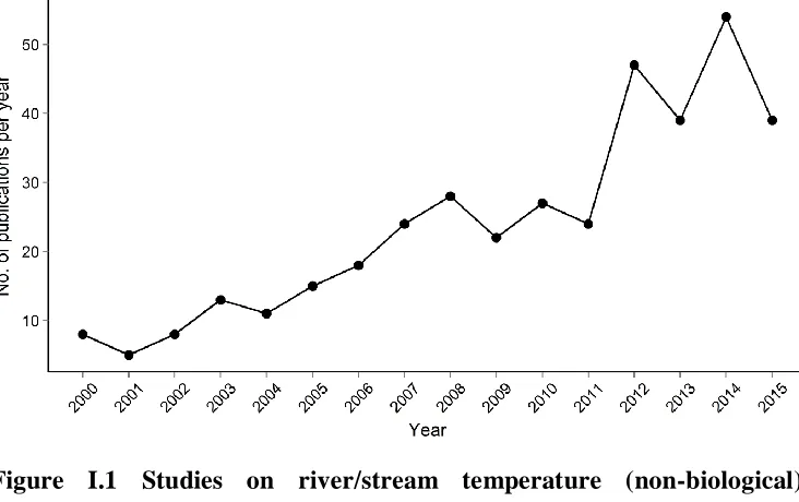
Figure I.1 Studies on river/stream temperature (non-biological) published since 2000. Publications were selected by searching within the ISI Web of Knowledge database using the key words: “stream temperature” OR “river temperature”.

1.2 Processes and controls determining river temperatures

(31)

4

net radiation is the dominant heat source to a river, accounting for more than 70% of heat inputs followed by sensible heat, while evaporation is the dominant sink (Hannah et al., 2004; Webb et al., 2008). However, at the sub-annual scale, the contributions change. During winters, net radiation is the dominant heat sink and sensible heat and bed conduction are the dominant energy sources (Hannah et al., 2004, 2008a). The various energy sources and sinks can be represented in a form of an equation, commonly known as the heat budget equation (Webb and Zhang, 1997) and has been the basis for several river temperature prediction models.

Controls of river temperature are defined by those variables which shape the natural thermal regime of a river via the above mentioned processes. These controls are multivariate and can be external or internal to the river system. External controls such as climate, runoff, highland vegetation, altitude and topographic shade, shape the river’s physical environment and control the rate of external heat and water inputs within the catchment. Internal controls such as channel and floodplain morphology, riparian buffer structure, and aquifer stratigraphy, define the river character and geometry, thereby, determining a channel’s resistance to warming or cooling and affecting the water temperature response to external temperature controls (Poole and Berman, 2001). These external and internal controls exert their influence over several spatial and temporal scales. Macroscale controls (> 100 km2; annual to monthly) such as climate, latitude, and altitude, drive the thermal regime of river. Mesoscale controls (100 km2- 100 m², monthly to daily) such as runoff volume and sources and basin aspect, modify the timing and magnitude of water temperature dynamics, and microscale controls (<100 m²; monthly to sub-daily) such as channel structure, topographic/riparian shading, hyporheic exchanges and groundwater inputs, further modify the sensitivity of river temperature to the local climate (Imholt et al., 2013; Hannah and Garner, 2015).

(32)

5

(Webb et al., 2008). The investigation of controls causing thermal heterogeneity at reach and site scale (vertical and lateral variation in water column) has been receiving renewed attention but needs further research, owing to the complexity of their interactions (Webb et al., 2008).

1.3 Changing river temperatures in changing environments and its implications

1.3.1 Changing river temperatures in changing environments: drivers of change

Humans have substantively altered the structure of river systems and the environmental setting along the course of rivers over time. Installation of dams, water withdrawals, modification of channel structure (e.g., straightening, bank hardening, diking), waste water inputs, the removal of vegetation (highland and riparian), and urbanization, are all examples of ways via which river temperature controls are altered. Global environmental changes, which include the aforementioned human modifications as well climate change, are, therefore, drivers of change of river temperature regimes (Hannah and Garner, 2015). These drivers of change, by modifying the magnitude and combination of controls, can alter the timing or the amount of net heat inputs into a channel, for e.g., by altering the amount of solar radiation (direct impact), and/or by affecting the flow regime of rivers (indirect impact). The resulting effect of these modifications depends on the sensitivity of rivers or their assimilative capacity for heat (such as rivers with low flows) (Poole and Berman, 2001), while such modifications can also alter a river’s sensitivity.

(33)

6

urbanization (LeBlanc et al., 1997; Nelson and Palmer, 2007; Hester and Bauman, 2013; Somers et al., 2013; Xin and Kinouchi, 2013; Booth et al., 2014). Increased air and land surface temperatures (up to 10°C), wastewater input, runoff from warmed impervious surfaces during precipitation, contribute to elevated river temperatures and heat surges within cities (Nelson and Palmer, 2007; Somers et al., 2013). River temperature changes in response to flow reductions (water abstractions) and releases below reservoirs have received increasing interest (Webb et al., 2008). Artificial reductions or increases in flow alter the assimilative thermal capacity of the river, resulting in an increased occurrence of high temperature events and increases in temperature minima, respectively (Webb et al., 2008; Hannah and Garner, 2015).

Drivers of change can also alter long-term river temperature dynamics. Recently, several studies have investigated the factors responsible for long-term changes in river temperature regimes. Majority of these studies have reported an increase in river temperature during the past decades (Hari et al.,

2006; Webb and Nobilis, 2007; Kaushal et al., 2010; van Vliet et al., 2011; Isaak et al., 2012; Markovic et al., 2013; Orr et al., 2014; Rice and Jastram, 2015), which have often been attributed to changes in air temperature. In some cases, long-term increase in river temperature have also been attributed to urbanization (Kinouchi et al., 2007), presence of dams (Petersen and Kitchell, 2001) as well as land use changes and water diversion (Arismendi

et al., 2012). Hence, there is a growing consensus on the fact that attribution of river temperature changes solely to climate change is difficult, given the simultaneous impacts of several drivers of change on river temperature. Additionally, as the different drivers of change act at several spatiotemporal scales, a generalization about the magnitude and the causes of river temperature change remains a challenge (Webb et al., 2008; Hannah and Garner, 2015).

1.3.2 Implications of changing river temperature on freshwater organisms

(34)

7

ultimately to river ecosystem health (Ormerod et al., 2010; Wooster et al.,

2012; Floury et al., 2013; Markovic et al., 2014). The observed increases in river temperature, especially when accompanied with altered flows, trigger various cascading effects on a number of physical, chemical and biological processes in river ecosystems (Pusch and Hoffmann 2000; Whitehead et al.,

2009) as well as on the physiology of freshwater biota and composition of communities. River warming has been shown to result in an earlier onset of adult insect emergence, increased growth rates, decreases in body size at maturity, altered sex ratios, decreased densities (Hogg and Williams, 1996), increased taxonomic richness (Jacobsen et al., 1997) and shifts in community structure of invertebrates (Daufresne et al., 2004; Durance and Ormerod, 2007; Haidekker and Hering, 2008). More recently, Woodward et al. (2010b) observed increases in food chain length with increasing water temperature, with fishes (e.g. brown trout) having a higher trophic status in warmer rivers as compared to colder rivers. Key ecosystem processes such as primary production and decomposition rates, also rise significantly with temperature (Bärlocher et al., 2008; Friberg et al., 2009) and consequently, affect other water quality variables such as decreases in dissolved oxygen levels (Johnson and Johnson, 2009). An increase in the frequency of extreme hydro-climatic events such as heat waves, droughts or floods can also have strong impacts on freshwater ecosystem processes and ecology. Both maximum temperatures and the frequency of warm spells (or heat waves i.e., at least five days of consecutively high maximum temperature) have increased between 1951 and 2010 and are assumed to increase further in the future (IPCC, 2013). Such events are likely to have profound and complex consequences for aquatic ecosystems (Lake, 2011) by causing loss of favourable habitat, limiting species dispersal, reducing resilience and causing local extinction of heat-sensitive taxa (Leigh et al., 2014).

(35)

8

Ormerod, 2009; Floury et al., 2013; Vaughan and Ormerod, 2014; Piggott et al., 2015). Particularly, as the interactive effects among increasing water temperature and other stressors are less explored (Woodward et al., 2010a; Piggot et al., 2015), there is a need to observe and quantify the impacts of multiple stressors (including water temperature) on the response of freshwater macroinvertebrate communities.

1.4 Research gaps, aims and structure of the thesis

Despite the rich literature on river temperature dynamics and the various factors controlling the dynamics, major research gaps remain, particularly with respect to spatial and temporal heterogeneity in river temperature (Webb et al., 2008; Hannah and Garner, 2015). At broad spatial and temporal scales, few studies have investigated past changes in river temperature and most of them have been carried out for North American rivers (Kaushal et al., 2010; Issak et al., 2012; Arsimendi et al., 2012; Caldwell et al., 2014; Rice and Jastram, 2015). In Europe, the most comprehensive study so far focused on river temperature trends at 2773 sites across England and Wales (Orr et al., 2012). Other studies on river temperature trends in Europe (e.g., Webb and Nobilis 1995; Hari et al.,

(36)

9

compared the relative impacts of increased water temperature, low flow and low DO levels on invertebrates by combined application of those stressors. More importantly, hardly any research on river temperature changes and dynamics has been done for German rivers. Markovic et al. (2013) quantified the variability, magnitude, and extent of temperature alterations at different time scales for 11 sites along the River Elbe and four sites along the River Donau in Germany, while Koch & Grünewald (2010) developed and assessed the performance of daily river temperature regression models for two stations on River Elbe. In Germany, the average annual air temperature has increased by about 1.3°C between 1881 and 2014 and the last 14 years have been the warmest so far (DWD, 2015). Also, average annual flow has increased for many rivers since 1950 (Bormann, 2010), mainly due to increasing winter flows, while summer flows have exhibited decreasing trends (Bormann, 2010; Stahl et al., 2010). Future climate projections predict significant warming across Germany with an increase in air temperature of 1.6 to 3.8°C by the year 2080 (Zeibsch et al., 2005). Moreover, extreme low flow conditions, especially in summer, are expected to become much more common, especially in eastern Germany (UBA, 2010; Huang et al., 2012). Finally, more than 90% of the rivers are in a moderate or bad ecological state (UBA, 2013), which makes it even more urgent to understand the past changes as well as the causes of spatiotemporal heterogeneity in river temperature behaviour and its role as a stressor.

Thus, this thesis aims to investigate spatial and temporal heterogeneity in river temperature at large and small scales for German rivers as well as the impact of increasing river temperature on freshwater invertebrates in a multiple stressor context. The specific aims and objectives of the thesis are as follows:

(37)

10

variables in inducing spatially and temporally variable river temperature changes.

2) Observe and quantify spatial variation in water temperatures in a lowland river and the role of landscape variables (Chapter 3): In this chapter, I observed spatial thermal heterogeneity in a ~200 km reach (20 sites) of a lowland river in northeast Germany (River Spree) for a period of nine months (January-September 2014) which flows through several land use types (forest, agricultural and urban areas). I quantified the heterogeneity in the heat budget and through a semi-empirical model and explored the role of hydro-climatological variables, land use types, lakes and river aspect in causing the observed thermal heterogeneity.

(38)

Chapter 2 Changing river temperatures in Northern Germany

11

2. Changing river temperatures in Northern

Germany: trends and drivers of change

Roshni Arora, Klement Tocknerand Markus Venohr

(Hydrological Processes,

(39)

Chapter 3 Reach scale thermal heterogeneity

38

3. Influence of landscape variables in inducing

reach-scale thermal heterogeneity in a lowland river

Roshni Arora, Marco Toffolon, Klement Tockner and Markus Venohr

3.1 Abstract

Identifying the role of landscape variables, especially land use, in inducing reach-scale thermal heterogeneity in river/stream temperature represents an ongoing task. The present study investigated the temporal and spatial heterogeneity of stream temperature (ST) and the role of landscape variables at 20 locations within a ~200 km reach of the intensively managed lowland river (River Spree) in northeast Germany over a 9-month period. The results showed the presence of thermal heterogeneity within the reach, which was most apparent during warmer months and was mainly affected by the presence of urban areas and lakes. Quantification of this effect in the heat budget was estimated via a residual heat flux term 𝐸_𝑟. Correlations of mean ST and 𝐸𝑟 with hydro-climatological and landscape variables at different

temporal and spatial extents corroborated the above results, showing that the influence of urban areas was independent of its distance from the river edge, at least within 1 km. Forest-induced microclimates also had a significant effect in moderating ST, but the effective spatial width was not clear. Furthermore, especially for lake influenced reaches, it was determined that the upstream advected heat determined the base ST, while climatological variations induced ST variations around that base temperature. Application of a semi-empirical model allowed for capturing the spatial heterogeneity in the reach and, as compared with regression models, delivered a much better performance in predicting ST with the same input data, questioning the widespread application of regression models.

3.2 Introduction

(40)

39

warmed in the past few decades (Kaushal et al., 2010; van Vliet et al. 2011; Isaak et al., 2012; Markovic et al., 2013; Rice & Jastram, 2015; Chapter 2) and are predicted to continue warming in the future (van Vliet et al., 2013). Increasing water temperature has detrimental impacts on water quality and habitat suitability for freshwater species, thereby having ecological as well as socio-economic consequences (EEA, 2008b; van Vliet et al., 2013). Large spatial heterogeneity in stream/river temperature could act as thermal migration barriers for freshwater species, reducing connectivity and harbouring different community compositions within the same reach (Sponseller et al., 2001; Kelleher et al., 2012). Accordingly, an increasing number of studies are being conducted to understand the controls of thermal dynamics of rivers, to delineate the causes of heterogeneity among systems and to identify the factors behind observed widespread river warming (Johnson et al., 2014).

Water temperature is a function of energy and hydrological fluxes at the air and riverbed interfaces of a river (Hannah and Garner, 2015). Heat is added to or lost from a river through mechanisms such as radiation, conduction, convection and advection (Webb and Zhang, 1997). In general, net radiation is the dominant source of heat to a river, accounting for more than 70% of heat inputs (Webb et al., 2008). Multiple controls (such as climate, flow, land use) can influence one or more of these processes at several spatiotemporal scales and induce thermal heterogeneity within and across river systems (Imholt et al., 2013; Hannah and Garner, 2015). The role of land use alteration in stream temperature modification, especially removal of forest canopy, has been explored extensively (Moore et al., 2005; Malcolm

(41)

40

directly or indirectly lead to creation of thermally heterogeneous reaches in rivers, by either altering the amount of incident solar radiation and/or by inducing different hydrologic responses in rivers (Poff et al., 2006; Sun et al., 2014). Most of the studies considering land use as an influencing factor or a determinant of stream temperature generally include forest as a variable (Pedersen and Sand-Jensen, 2007; Hrachowitz et al., 2010; Broadmeadow et al., 2011; Mayer, 2012; Imholt et al., 2013; Hebert et al., 2014), whereas only few have studied the effect of other land use types in causing different river thermal environments. For example, Chang et al. (2013) found percent share of forest cover to be a better predictor of maximum stream temperature in Columbia River basin than urban, agriculture or grassland cover. A modelling study by Sun et al. (2014) also found that reforestation of an urbanized area had a more pronounced effect on stream temperature than urbanization of a forested area, suggesting a dominant influence of riparian vegetation. Kaushal et al. (2010) and Rice and Jastram (2015) suggested more rapid long-term increases in stream temperature in urban areas than in other land use types for several North American rivers. Also, thermal sensitivity of small urban streams has been observed to be higher than of rural or forested streams in Pennsylvania (Kelleher et al., 2012). However, majority of these studies have been conducted at large spatial scales (basin/watershed). To our knowledge, no study has yet investigated within-stream or reach-scale heterogeneity in water temperature of a river flowing through different land-use types. Hence, understanding drivers of thermal heterogeneity in watercourses over a range of scales still presents an ongoing challenge (Webb et al., 2008).

(42)

41

observations towards the lower end of major river systems (Broadmeadow et al., 2011). We specifically addressed the following questions:

1) Is there any spatial heterogeneity in stream temperatures (ST) along the reach and, if present, can it be quantified in the heat budget? 2) Is the observed spatial thermal heterogeneity related to the spatial

location of land use types along the reach? At what temporal scale (daily, monthly, entire period) and lateral spatial extent is the impact of land use types most apparent?

3) How do other landscape variables such as lakes or stream aspect and hydro-climatological variables contribute to the thermal heterogeneity?

4) How well can a semi-empirical model capture the dominant controls of ST in the reach?

In addition, given the need to move beyond regression models owing to their poor performance (Arismendi et al., 2014), we also compared the performance of regression models with a semi-empirical hybrid model in predicting stream temperature (Toffolon and Piccolroaz, 2015), based on air temperature as input.

3.3 Materials and methods

3.3.1 Study area

(43)

42

bedrock in most of the catchment, the flow regime of the Spree is highly deteriorated in comparison to other rivers of similar size in Central Europe. The mean discharge for the year 2014 near Fehrow was 4 m3s-1 whereas near Spandau it was 23 m3s-1. The specific runoff between Cottbus and Berlin ranged from 2.4 - 4.1 L km-2 s-1 during 1997-2007 (Tockner et al., 2009). The annual discharge regime is regulated and smoothed by reservoirs in the upper part and weirs immediately downstream of lakes and in smaller tributaries. Majority of the lakes and reservoirs in this region are shallow and have low landscape gradients (Kozerski et al., 1991).

Climate in the entire catchment is mostly sub-continental with relatively low annual precipitation and hot and dry summers. Mean annual temperature at Lindenberg, which is in the middle of the lower catchment, was 9.2°C (time period 1981-2010). It is one of the driest regions within Germany with precipitation up to 500 mm (below 576 mm in the period 1981-2010 at Lindenberg).

Despite low water availability in the catchment, this lower section of River Spree has multiple uses, such as drinking water supply, recreation, coolant for power plants, receiving tertiary-treated wastewater, waterway for navigation, and is thereby subject to several pressures. Also, it has undergone severe transformations due to lignite mining activities in the past, making it one of the most intensively managed rivers of the world (Tockner et al.,

(44)

43

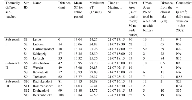
Figure III.1 Maps showing the location of the study area, stream temperature (ST) measuring locations, and the thermally heterogeneous sub-reaches. Stream temperature measuring locations are numbered corresponding to their IDs (Table III.2).

3.3.2 Dataset

(45)

44

(available for all loggers) were used, whereas for model applications entire year’s data were used where available.

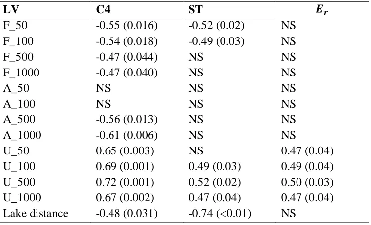
Table III.1 Hydro-climatological and landscape variables considered in the analysis.

Hydro-climatological

variables Landscape variables

Air temperature [°C] Forest area in 50 m buffer (F_50) [%] Solar radiation [J cm-2] Forest area in 100 m buffer (F_100) [%] Relative humidity [%] Forest area in 500 m buffer (F_500) [%] Wind velocity [m s-1] Forest area in 1000 m buffer (F_1000) [%] Atmospheric pressure [mbar] Agricultural area in 50 m buffer (F_50) [%] Cloud cover [okta] Agricultural area in 100 m buffer (F_100) [%] Discharge [m s-3] Agricultural area in 500 m buffer (F_500) [%]

Agricultural in 1000 m buffer (F_1000) [%] Urban area in 50 m buffer (F_50) [%] Urban area in 100 m buffer (F_100) [%] Urban area in 500 m buffer (F_500) [%] Urban area in 1000 m buffer (F_1000) [%] Lake distance [m]

Stream azimuth (aspect) [°]

(46)

45

(LUGV; www.luis.brandenburg.de/) and were available at six locations within the study reach (Fig. III.1).

A total of 14 landscape variables were included in the study and basically comprised of shares (%) of land cover for different buffer widths, lake distance and stream azimuth (aspect) (Table III.1; Fig. SIII.1). Land cover data along the reach were obtained from ATKIS land-use dataset (10 m × 10 m resolution; ADV, Germany). Lake distances and stream azimuth values were calculated from Google Earth. Azimuth was measured as the angle (degrees) that the overall stream channel differed from due south (e.g., due south = 0°, due west = +90°, and due east = -90°) (Arscott et al., 2001). Since elevation was very similar across sites (58-30 m), it was not considered for analysis.

3.3.3 Quantification of contribution of landscape controls in the heat budget

Heat content variations in a river reach was computed using the following energy balance:

𝑑

𝑑𝑡(𝜌 𝐶𝑝 𝑉 𝑇𝑤) = 𝐻𝑢𝑝− 𝐻𝑑𝑜𝑤𝑛+ 𝑆 (𝐸𝑎𝑡𝑚+ 𝐸𝑟+ ∆𝐸) (1)

where 𝑇𝑤 is stream temperature, 𝜌 and 𝐶𝑝 are density (assumed constant, 997

kg m-3) and specific heat of water (assumed constant, 4179 J kg-1 °C-1), 𝑉 is volume of the reach (m3), 𝑆 is the surface area (m2), 𝐻_𝑢𝑝 is the total heat flux entering (W) the volume from the upstream section, 𝐻_{𝑑𝑜𝑤𝑛} is the total heat flux (W) going out downstream, 𝐸atm is the net exchange per unit surface (W

m-2) with atmosphere estimated as an average value for the whole study area. The various heat flux components of 𝐸atm (solar radiation, sensible and

(47)

46

values were region-based and not site-based, effects of reduced incident solar radiation (reduced heat inputs) in shaded areas are also included in 𝐸_𝑟.

Equation (1) was discretized by subdividing the entire reach into computational reaches defined by the location of the ST measuring sites. Each computational reach had a discrete stream temperature 𝑇_𝑤,𝑖𝑘 (°C, with 𝑖 the index for space and 𝑘 for time) in the volume 𝑉_𝑖. Assuming steady and uniform hydraulic conditions (i.e., constant discharge, Q (m3 s-1), or/and cross-section) along a computational reach 𝑖, and further assuming that the downstream temperature 𝑇_{𝑤,𝑑𝑜𝑤𝑛}≅ 𝑇_𝑤,𝑖𝑘 (thus considering each computational reach as a completely mixed reactor), the upstream and downstream heat fluxes were calculated as 𝐻_𝑢𝑝 = 𝜌𝐶_𝑝𝑄_𝑖𝑇_{𝑤,𝑖−1} and 𝐻_{𝑑𝑜𝑤𝑛} = 𝜌𝐶𝑝𝑄𝑖𝑇𝑤,𝑖, respectively. Thus, the temperature change in a river reach can be

calculated by the following heat balance:

𝑇_𝑤,𝑖𝑘+1−𝑇_𝑤,𝑖𝑘

∆𝑡 =

𝑄𝑖

𝑉𝑖 (𝑇𝑤,𝑖−1

𝑘 _{− 𝑇}

𝑤,𝑖𝑘 ) + 𝑆𝑖𝐸𝑎𝑡𝑚_{𝜌 𝐶}+ ∆𝐸

𝑝 𝑉𝑖 + 𝑆𝑖

𝐸𝑟,𝑖

𝜌 𝐶𝑝 𝑉𝑖 , (2)

where, an explicit Euler scheme was used for the discretization, as a first approximation. The volume was estimated as 𝑉𝑖 = 𝐵𝑖𝐷𝑖𝐿𝑖, where 𝐵𝑖 is the

river width (m), 𝐷_𝑖 is the depth (m) and 𝐿_𝑖 the length (m) of the reach. All the surface heat fluxes were calculated referring to a surface area 𝑆𝑖 = 𝐵𝑖𝐿𝑖.

Alternatively, if the temperature changes across space and time are known, equation (2) yields a way to estimate the residual heat term,

𝐸_𝑟,𝑖 = 𝜌 𝐶_𝑝 𝐷_𝑖 (𝑇𝑤,𝑖𝑘+1−𝑇𝑤,𝑖𝑘

∆𝑡 ) − 𝜌 𝐶𝑝 𝑄_𝑖

𝐵𝑖𝐿𝑖 (𝑇𝑤,𝑖−1

𝑘 _{− 𝑇}

𝑤,𝑖𝑘 ) − 𝐸𝑎𝑡𝑚− ∆𝐸 (3)

(48)

47

assumed to be negligible. Ultimately, 𝐸_𝑟 mainly consists of heat contributions from land-use sources and lake inflows (the latter by means of alterations of the upstream heat flux) within the reach.

(49)

48

Table III.2 Description of the stream temperature observation sites on River Spree.

Thermally different sub-reaches Site ID

Name Distance

(km) Mean ST for entire period Maximum ST (15 min) Time at Maximum ST Forest Area (% of total in reach; 50 m wide buffer) Urban Area (% of total in reach; 50 m wide buffer) Distance from the closest lake (km) Conductivit y

(μ cm-1 ; daily mean value on 14 Jan 2008) Sub-reach I

S1 Leipe 0 13.04 24.25 21-07 17:15 30 16 51 947

S2 Lubben 14 13.06 24.87 21-07 17:30 62 17 65 857

S3 Hartmannsdorf 18 13.14 25.26 21-07 17:00 32 50 69 822

S4 Schlepzig 27 13.25 25.30 22-07 18:00 92 2 78 NA

S5 Leibsch 33 13.32 25.26 22-07 18:15 33 5 84 815

Sub-reach II

S6 Altschadow 42 13.95 27.78 20-07 15:00 13 10 0.5 893

S7 Werder 49 13.90 26.83 21-07 02:15 19 1 8 NA

S8 Kosenblatt 52 13.73 27.08 21-07 15:00 23 6 11 NA

S9 Trebatsch 62 13.77 26.37 21-07 23:15 22 7 21 0.88

Sub-reach III

S10 Radinkendorf 81 14.13 26.88 21-07 16:15 41 13 2 823

S11 Rassmansdorf 87 14.03 26.41 21-07 16:30 25 2 8 0.84

S12 Drahendorf 99 13.80 25.77 20-07 16:15 35 3 10 837

(50)

49

S14 Furstenwalde 116 13.97 26.79 20-07 15:00 35 65 27 836

S15 Hangelsberg 129 13.73 26.34 22-07 13:15 38 7 40 NA

S16 Freienbrink 141 13.81 26.42 20-07 19:00 21 3 52 NA

S17 Neu zittau 148 13.24 24.79 20-07 18:00 15 9 59 832

Sub-reach IV

S18 Warschauer str 176 14.14 26.59 20-07 18:00 33 53 16 NA

S19 Jannowitz 179 14.18 26.63 20-07 15:00 0 100 19 824

(51)

50

3.3.4 Identification of dominant ST controls

3.3.4.1 Lagrangian model

In order to ascertain the mechanism through which the upstream conditions affect downstream ST and the role of riparian buffer in regulating water temperature, we developed a simple Lagrangian model (Leach and Moore, 2011). In this approach, a reach is divided into a series of segments bounded by nodes (index 𝑗). A water parcel having an initial ST (based on measured values) is released from the upstream boundary at each time step. As the water parcel flows downstream from one node to the next (𝑗 to 𝑗 + 1), the model computes the heat inputs and the consequent change in stream temperature over the stream segment. This can be formally represented as follows:

𝑇_𝑤(𝑥_𝑗+1, 𝑡_𝑘+1) = 𝑇_𝑤(𝑥_𝑗, 𝑡_𝑘) + (𝜌 𝐶_𝑝 𝐷_𝑗)−1∑ 𝐸_𝑙 ∆𝑡 , 𝑥_𝑗+1 = 𝑥_𝑗+ 𝑈_𝑗∆𝑡, (4)

where, ∑ 𝐸𝑙= 𝐸𝑎𝑡𝑚+ 𝐸𝑟+ ∆𝐸 represents the sum of all the external heat

fluxes acting in the time interval ∆𝑡 (15 min). In our simulation, the flow velocity 𝑈𝑗 was assumed as constant in each segment 𝐿𝑖. Reference values of

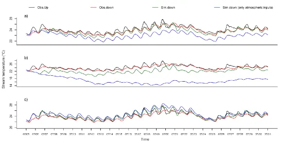
flow velocity 𝑈 = 0.2 m/s and depth 𝐷 = 1 m were estimated by steady-state simulations using the software HEC-RAS (USACE, 2010; http://www.hec.usace.army.mil). The hydrodynamics of the river was characterized assuming a simplified geometry of equivalent rectangular cross-sections having width 𝐵 = 40 m, as the information on the longitudinal variation of the cross-sections of the river was insufficient. For this analysis, the STs were simulated for site S9 (downstream) starting from the upstream site S6 (located at a lake outlet), for 15 days in July (5/07-31/07), the hottest month of the year.

To determine the influence of upstream conditions, simulations using the Lagrangian model were compared with the simulations from a reduced model based on equation (2) with ST determined locally (hereafter termed “local” Eulerian model) at a site 𝑖:

𝑇𝑤(𝑥𝑖, 𝑡𝑘+1) = 𝑇𝑤(𝑥𝑖, 𝑡𝑘) + (𝜌 𝐶𝑝 𝐷𝑗)−1∑ 𝐸𝑙 ∆𝑡 , (5)

(52)

51

regulating ST below lakes, STs were simulated using the Lagrangian and the “local” Eulerian model in two scenarios of incident solar radiation inputs, zero (complete shade) and 100% (no shade).

3.3.4.2 Correlations, linear and non-linear statistical modelling

Statistical analyses to describe different aspects of stream thermal dynamics where performed on the basis of mean daily and mean monthly values. To estimate daily contributions of hydro-climatological variables in ST variations at each site, linear regression and generalized non-linear models (spline-smoothing function from the mgcv package in R software, where significance of the smooth term was reported) were applied to daily values of ST and hydro-climatological variables. The Durbin–Watson test was used to detect autocorrelation in the linear model residuals and was found to be significant for all variables. In the presence of autocorrelation, the reported R2 statistics should be interpreted as an upper limit since autocorrelation tends to reduce the sample sizes of the regression models (Johnson et al., 2014). Logistic regression model (Mohseni et al., 1998) was also fitted to air temperature and ST values to compare with linear regression model performance according to the following equation:

𝑇𝑤= 𝜇 +_1+𝑒𝛼−𝜇_{𝛾(𝛽−𝑇𝑎)} , (6)

where 𝑇𝑤 is the estimated water temperature, 𝑇𝑎 is the measured air

temperature, α is the estimated maximum water temperature, µ is the estimated minimum water temperature, γ is a measure of the slope between water and air temperature, and β represents the inflexion point of the curve. Mean and maximum values of ST (at daily/monthly/entire period time scales) and mean values of 𝐸𝑟 (monthly/entire period time scales) were used

to calculate Pearson’s correlations for the analysis of the role of landscape variables in modifying ST on a reach scale.

3.3.4.3 Semi-empirical hybrid model

(53)

52

approach to relate ST to air temperature was applied based on the same input variables. The air2stream model (Toffolon & Piccolroaz, 2015) represents an adaptation (for rivers) of the air2water approach that was successfully applied to predict lake surface temperature as a function of air temperature (Piccolroaz et al., 2013; Toffolon et al., 2014; Piccolroaz et al., 2015). It is based on a lumped heat budget that considers an unknown volume of the river reach, its tributaries (implicitly considering both surface and subsurface water fluxes), and the heat exchange with the atmosphere. The heat budget (equation 1) is simplified until only the dependency on air temperature (as a proxy of the other processes) is retained (please refer to Toffolon and Piccolroaz, 2015 for further details). The model is proposed in five versions, each based on different assumptions, and the versions differ for the number of parameters (from 3 to 8). The 8-parameter version is the full model and incorporates the contribution of discharge. Since the discharge data were not available at all locations, the 5-parameter version of the model was used for this analysis:

𝑑𝑇_𝑤

𝑑𝑡 = 𝑐1+ 𝑐2𝑇𝑎− 𝑐3𝑇𝑤+ 𝑐4cos [2𝜋 ( 𝑡

𝑡_𝑦− 𝑐5)] , (7)

where 𝑇𝑤 is the stream temperature, 𝑇𝑎 is the air temperature, t is time (in

days), 𝑡_𝑦 is the duration of a year (in days) and 𝑐₁ to 𝑐₅ are constant parameters (corresponding to 𝑎₁, 𝑎₂, 𝑎₃, 𝑎₆, and 𝑎₇ of the original formulation in Toffolon and Piccolroaz, 2015). The values of these parameters are estimated through calibration, so that neither the geometrical characteristics of the river reach (length, volume, area, etc.) nor the roles of specific heat inputs (e.g., internal friction, along-reach inflows) are explicitly specified. The second term on the right hand side of equation (7) represents the effect of air temperature (as a proxy) on the net heat flux. The fourth term on the right hand of equation represents the heat fluxes associated with inflows, representing the contribution of factors (such as groundwater, land use, lakes) which modify ST dynamics but are of difficult determination. If we divide equation (6) with the coefficient of 𝑇𝑤, 𝑐3, we obtain

𝐶3𝑑𝑇_𝑑𝑡𝑤= 𝐶1+ 𝐶2𝑇𝑎− 𝑇𝑤+ 𝐶4cos [2𝜋 (_𝑡𝑡

(54)

53

where 𝐶₃= 1 𝑐⁄ ₃, and 𝐶_𝑛= 𝑐_𝑛⁄𝑐₃ (𝑛 = 1, 2, 4). If 𝐶₃, which is the time scale for adaptation of ST to local conditions, is small enough, then the left hand term will stand for instantaneous adaptation, hence explicitly providing the equilibrium temperature (Toffolon and Piccolroaz, 2015): 𝑇_{𝑤,𝑒𝑞}= 𝐶₁+ 𝐶₂𝑇_𝑎+ 𝐶₄𝑐𝑜𝑠[2𝜋(𝑡 𝑡⁄ − 𝑐_𝑦 ₅)] . Parameters 𝐶₂ and 𝐶₄ are the measures of sensitivity to air temperature and contribution of unresolved seasonal inflows, respectively.

Differently from other applications of air2stream (e.g., Toffolon and Piccolroaz, 2015; Piccolroaz et al., submitted), because of the short ST record (January-December 2014; including missing values where present), here, the parameters of equation (7) were calibrated using the entire dataset without an independent validation.

3.4 Results

3.4.1 Spatial and temporal variation in stream temperature

(55)

54

The entire ~200 km study reach can be segregated into four sub-reaches which are thermally heterogeneous from each other (Fig. III.1; Table III.2). Sub-reach I flows through a mix of forested and agricultural area with interspersed urban areas in some regions; sub-reach II is majorly dominated by agricultural area; sub-reach III flows through mostly semi-forested/agricultural areas; and sub-reach IV is situated within the Berlin city. The site S17 (within sub-reach III) was a bit peculiar, being much cooler than rest of the sites in sub-reach III during April-July and warmer during January. This could be an indication of a probable local influence of groundwater or the logger might have come in close contact with the riverbed. During summer, a downstream cooling trend within sub-reaches II and III (except warming at S14) was very apparent (Fig. III.2). Across sub-reaches as well, the ST increased downstream, with each sub-reach being warmer than its upstream sub-reach. During winter, the ST decreased downstream, with hardly any differences between sub-reaches II and III (Fig. III.2).

(56)

55

Figure III.2 Daily means for the 4th (blue), 10th (dark green) and 15th (black) day of each month plotted for the 20 sites on River Spree for all months during the study period.

3.4.2 Spatiotemporal variation in the contribution of the ‘other’ heat fluxes

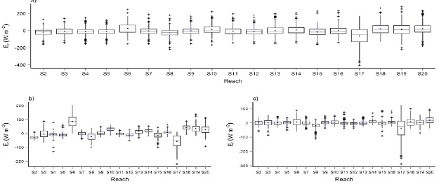
The residual energy flux term 𝐸_𝑟 denotes the unresolved contribution of heat flux within a reach via sources other than exchange with the atmosphere, for

e.g., due to factors such as land use and inflows from lakes (within the reach), tributaries, groundwater and/or wastewater. The mean 𝐸_𝑟 for the study period was positive (and highest) for sites at lake outlets and/or within urban areas (namely, S6, S10, S14, S18, S19 and S20), signifying that ‘other’ sources were a heat source within reaches upstream of these sites (Fig. III.3a). The 𝐸𝑟 term remained positive for up to 52-63% of the entire

study period for these sites. At the other sites, either the absence of these inputs or the presence of forested areas caused 𝐸𝑟 to be negative, implying

(57)

56

S10, S14, S18, S19 and S20 at the downstream end was received during warmer months (June to Sep) (Fig. III.3b, c).

(58)

57

(59)

58

(60)

59

3.4.3 Dependence on hydro-climatological and landscape variables

3.4.3.1 Correlations with hydro-climatological variables

(61)

60

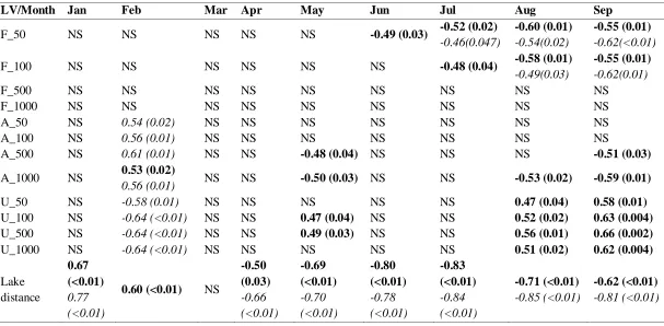
Table III.3 Correlations of parameter C4 (air2stream), mean stream temperature (for the entire period), mean 𝑬_𝒓(for the entire period) with landscape variables (LV). NS stands for not significant correlations.

LV C4 ST 𝑬𝒓

F_50 -0.55 (0.016) -0.52 (0.02) NS

F_100 -0.54 (0.018) -0.49 (0.03) NS

F_500 -0.47 (0.044) NS NS

F_1000 -0.47 (0.040) NS NS

A_50 NS NS NS

A_100 NS NS NS

A_500 -0.56 (0.013) NS NS

A_1000 -0.61 (0.006) NS NS

U_50 0.65 (0.003) NS 0.47 (0.04)

U_100 0.69 (0.001) 0.49 (0.03) 0.49 (0.04)

U_500 0.72 (0.001) 0.52 (0.02) 0.50 (0.03)

(62)

61

(63)

62 3.4.3.2 Correlations with landscape variables

Stream temperature: Several significant correlations of ST metrics with landscape variables were detected at monthly, daily scales as well as for the entire time period. Over the study period, share (%) of urban and forest area in >50 m and ≤100 m wide buffers, respectively, were significantly correlated with the mean STs (Table III.3). At the monthly scale, significant correlations of land use shares with mean STs were observed mostly for warmer months (May-Sep) (Table III.4). Share of forest area within 100 m had a significant negative correlation with both mean and maximum monthly STs. On the other hand, share of urban area showed strong significant correlations with mean monthly STs during warm months (positive) and with maximum monthly STs during February (negative), irrespective of the buffer width (Table III.4). Share of agricultural area was also significantly correlated with mean monthly STs during warm months (≥500 m) and with maximum monthly STs during February (all buffer widths). At the daily scale, share of forest cover within 50 m and urban cover within 500 m had the highest number of significant correlations with mean ST (44% of 259 days) as well as with maximum ST (forest (50 m): 38%; urban (500 m): 36%).

Distance from lakes had a significant negative correlation with the mean ST for the study period (Table III.3). At the monthly scale, mean and maximum STs of warmer months had a significant negative correlation with lake distance, while a significant positive relationship was observed during the coldest months (Table III.4). At the daily scale, significant correlations of lake distance with mean and maximum STs were similar in number (mean = 73.7%; max = 72.2%). No significant correlations between stream azimuth and ST were detected at any time scale.

(64)

63

(65)

64

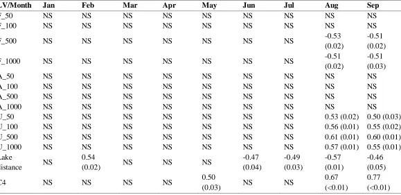
Table III.4 Significant correlations between landscape variables (LV, see Table III.1) and mean (bold), maximum (italic) monthly STs for all sites. NS stands for “not significant” correlations. P-values for significant correlations are provided within the brackets.

LV/Month Jan Feb Mar Apr May Jun Jul Aug Sep

F_50 NS NS NS NS NS -0.49 (0.03) -0.52 (0.02)

-0.46(0.047)

-0.60 (0.01) -0.54(0.02)

-0.55 (0.01) -0.62(<0.01)

F_100 NS NS NS NS NS NS -0.48 (0.04) -0.58 (0.01)

-0.49(0.03)

-0.55 (0.01) -0.62(0.01)

F_500 NS NS NS NS NS NS NS NS NS

A_50 NS 0.54 (0.02) NS NS NS NS NS NS NS

A_100 NS 0.56 (0.01) NS NS NS NS NS NS NS

A_500 NS 0.61 (0.01) NS NS -0.48 (0.04) NS NS NS -0.51 (0.03)

A_1000 NS 0.53 (0.02)

0.56 (0.01) NS NS -0.50 (0.03) NS NS -0.53 (0.02) -0.59 (0.01)

U_50 NS -0.58 (0.01) NS NS NS NS NS 0.47 (0.04) 0.58 (0.01)

U_100 NS -0.64 (<0.01) NS NS 0.47 (0.04) NS NS 0.52 (0.02) 0.63 (0.004) U_500 NS -0.64 (<0.01) NS NS 0.49 (0.03) NS NS 0.56 (0.01) 0.66 (0.002)

U_1000 NS -0.64 (<0.01) NS NS NS NS NS 0.51 (0.02) 0.62 (0.004)

Lake distance 0.67 (<0.01) 0.77 (<0.01)

0.60 (<0.01) NS

(66)

65

Table III.5 Significant correlations between landscape variables (LV, see Table III.1) and mean monthly 𝐄_𝐫 for all sites. NS stands for “not significant” correlations. P-values for significant correlations are provided within the brackets.

LV/Month Jan Feb Mar Apr May Jun Jul Aug Sep

F_500 NS NS NS NS NS NS NS -0.53

(0.02)

-0.51 (0.02)

F_1000 NS NS NS NS NS NS NS -0.51

(0.02)

-0.51 (0.03)

A_50 NS NS NS NS NS NS NS NS NS

U_50 NS NS NS NS NS NS NS 0.53 (0.02) 0.50 (0.03)

Lake

distance NS

0.54

(0.02) NS NS NS

-0.47 (0.04) -0.49 (0.03) -0.57 (0.01) -0.46 (0.05)

C4 NS NS NS NS 0.50

(0.03) NS NS

0.67 (<0.01)

(67)

66

3.4.4 Evaluation of the semi-empirical model versus regression models with air temperature as input

3.4.4.1 Regression models

The overall performances of the regression models are in general not satisfactory. Linear regression models showed a poor performance with the root mean square error (RMSE) varying from 2.4°C to 3.3°C, with a general tendency of worsening downstream (Fig. III.6). Logistic models fared better than the linear models, given the non-linear (s-shaped) relationship of air temperature with ST. The performance of logistic regression model also worsened downstream, with the RMSE increasing from 1.6°C to 2.4°C (Fig. III.6).

Figure III.6 Root Mean Square Errors (RMSE) for the three models for all sites on River Spree.

3.4.4.2 Semi-empirical hybrid model