RETRACTED ARTICLE: Is it possible to control and optimize technology transfer process?

R E V I E W

Open Access

Is it possible to control and optimize technology

transfer process?

Stefano De Falco

Abstract

Is it possible to control and optimize technology transfer process? Engineers and quality practitioners are often faced with the problem of determining the optimal choice of key factor in the tolerance process evaluation regarding the quality of the process to be monitored. To guarantee a prefixed quality level of the monitored process, lower specification limit (LSL) and upper specification limit (USL) for a certain quality characteristic have been determined. These limits, LSL and USL, could be defined asμ−δσandμ+δσ, respectively, whereδ>0. Here, the key factorδrepresents the number of standard deviations at which each specification limit is located from the process mean. This paper shows an innovative use of SPC tools in a different field aspect, one in which they are usually employed. Generally, these instruments are used for the control of the industrial process or service, but they could be used in an innovative way to control and to optimize a particular process: the technology transfer process. When determining the key factor level, it is important to consider a trade-off between costs incurred by the supplier, in terms of technology offer, and the user, in terms of technology request, of the process examined. This paper shows how these costs are quantified and integrated; it also shows how a particular mathematical tool, the Lambert W function, is incorporated into this choice optimization problem by deriving a closed-form solution. This proposed model and solution may be appealing to managers and technology transfer operators since the Lambert function is found in a number of standard optimization software. Experimental results are presented and related to a real data set of technology transfer actions developed by the Technology Transfer Office.

Keywords:Technology transfer, Numerical tools, Cost analysis

Review Introduction

The study on technology transfer covers various disciplines and topics such as the process, the barriers, the opportunities, and the modes of technology transfer (Reisman 2005). Functional performance and economic considerations should be considered in this analysis as driving factors affecting the choice of key factor in the quality analysis of a technology transfer (TT) process. A tight standard deviation in a generic process usually im-plies high cost (for example, high manufacturing cost) due to additional (manufacturing) operations, slow processing rates, additional care on the part of the operator, and a need for expensive measuring and processing equipment. The functional performance, however, can be improved by

specifying a tight standard deviation on a quality character-istic. On the other hand, a wide standard deviation reduces the (manufacturing) cost but may considerably lower the material quality level. Thus, determining optimal standard deviation involves a trade-off between the level of quality based on functional performance and the costs associated with the standard deviation. In this particular context, the manufacturing cost could be assimilated to knowledge production. In order to facilitate the economic trade-off, it is possible to express quality in monetary terms using a quality loss function. The quadratic loss function is widely used in the literature as a reasonable approximation of the actual loss to the customer due to the deviation of product performance from its target value. By expressing the level of quality in monetary terms, the problem of trading off quality with costs is converted into a problem of minimiz-ing the total cost, which is the sum of quality loss and costs. The costs associated with the standard deviation in-clude rejection, inspection, and manufacturing costs. Correspondence:[email protected]

Technology Transfer Magazine, Italian Association for Promotion of Culture of Technology Transfer, Technology Transfer Office, School of Sciences and Technologies, University of Naples, Federico II, Via Cinthia, Naples 80 126, Italy

© 2012 De Falco; licensee Springer. This is an Open Access article distributed under the terms of the Creative Commons Attribution License (http://creativecommons.org/licenses/by/2.0), which permits unrestricted use, distribution, and reproduction in any medium, provided the original work is properly cited.

The problem of determining an optimal level of toler-ance is equivalent to the problem of determining opti-mal specification limits since the term refers to the distance between its lower specification limit (LSL) and upper specification limit (USL).

Behind the different object of the application's method-ologies regarding the technology transfer process, the pro-posed analysis in this paper also differs from previous studies of optimization of choice of the key factor in two ways. First, a more general optimization model is pro-posed by simultaneously considering the quality loss in-curred by the user, and manufacturing and rejection costs incurred by the manufacturer in a building process, than a numerical example, relate to a specific process (TT process) that will be developed. Second, this paper shows how the Lambert W function, widely used in physics, can be efficiently applied to the optimization problem, which may be the first attempt in the literature related to optimization and synthesis. There are two significant bene-fits from using the Lambert W function in the context of choice of key factor optimization. Most optimization mod-els require rigorous optimization processes using numer-ical methods since closed-form solutions are rarely found. Using the Lambert W function, TT practitioners and re-search and development (R&D) managers cannot only ex-press their solutions in a closed form, but they can also quickly determine their optimal choice without resorting to numerical methods since a number of popular mathem-atical softwares, including MapleW and MatlabW, contain the Lambert W function as an optimization component.

Literature review

There are not many previous studies about the opportun-ity to transpose such models, methodologies, and tools from the quality field to the TT field. Robinson (1988) has identified a large number of factors and sub-factors that are relevant to the international technology transfer process. This model does not include any prescription for successful transfer. Keller and Chinta's (1990) integrative model, however, provides some strategic guidelines for this purpose. Although this model focuses on the success of the transfer process, there is no discussion on the post transfer performance of the technology.

Sarina et al. (2009) refer to technology transfer perform-ance through the research of relationship between the technology transfer itself and the absorptive capacity. Quazi (1998) illustrates the application of the principles in total quality management to the International Technology Transfer processes used in industrial production plants.

While regarding the studies on the use of the Lambert function in the traditional sectors of application, a num-ber of researchers have considered the problem of deter-mining optimal tolerance.

Chase et al. (1990) and Kim and Cho (1999) investi-gated the effect of tolerances on manufacturing cost and proposed models to determine tolerances for the minimization of manufacturing cost. Fathi (1990), Phil-lips and Cho (1999), and Kim and Cho (2000) studied the issue of tolerance design from the viewpoint of functional performance, where functional performance is expressed in monetary terms using the Taguchi quality loss concept (Taguchi 1986). Tang and Tang (1989) discussed an eco-nomic model for selecting the most profitable tolerance in a complete inspection plan for the case where inspec-tion cost is a linear funcinspec-tion of the tolerance. Fathi (1990) devised a graphical approach for determining tol-erances to minimize the quality loss and rejection costs for a single quality characteristic. Other studies (Tang 1991; Tang and Tang 1994) further investigated screening inspection for multiple performance variables in a serial production process. Tang (1988) presented a comprehen-sive literature review related to the design of screening procedures. Jeang (1997) proposed an optimization model for the simultaneous optimization of manufactur-ing and rejection costs and quality loss usmanufactur-ing a process capability index to establish a relationship between the tolerance and standard deviation. The model assumes a zero process bias condition, that is, the mean is equal to the target value for the quality characteristic. Further, the ratio of tolerance to the standard deviation is assumed to be constant. Jeang (1999) demonstrated how response surface methodology can be employed to determine tol-erances of components in an assembly. Kapur (1988) considered a tolerance optimization problem using

trun-cated normal, Weibull, and multivariate normal

distributions.

The Lambert W function: a brief overview

Lambert considered the trinomial equation x¼aþxb

by giving a series development for x in powers of a

(Chase et al. 1990). This equation can be transformed into a more symmetrical form:

xαþxβ¼ðαβÞvxαþβ ð1Þ

by substituting xβ for x and setting b¼αβ and a¼

αβ

ð Þv. Dividing Equation 1 by ðαβÞ and letting β converge toα, Equation 2 is obtained:

logx¼vxα ð2Þ

Lambert's generalized series solution for xn _{is given as}

follows:

xn_¼1þnvþ1

2n nð þαþβÞv

2_þ1

6n nð þαþ2βÞðnþ2αþβÞv

3_þ

þ1

24n nð þαþ3βÞðnþ2αþ2βÞðnþ3αþβÞv

4_{þ. . .}

Using the series given by Equation 3, Corless et al. (1996) show that Equation 2 can be written as:

logx¼vþ2

1

2!v 2_þ32

3!v 3_þ43

4!v 4_þ54

5!v

5_{þ ð4Þ}

This series shown in Equation 4 converges to Lambert

W(z), which is defined as follows:

LambertW zð ÞeLambertW zð Þ¼z ð5Þ

The Lambert W function is defined to be a multi-valued inverse of the functionð Þ ¼z zez_{, that is, Lambert}

W(z) can be any function that satisfies Equation 5 for all

z. This function allows solving such functional equations as g zð Þeg zð Þ _{¼z and ð Þ ¼z e}W ln zð ð ÞÞ_{, and ze}z _{¼x and z¼}

W xð Þ.

Determining optimal choice of key factor

One index that could be used as representative of TT process performance is the number of invention disclo-sures. This index is considered by Hulsebeck as ‘the most important measurable performance indicator of TTO’(Hulsebeck et al. 2011).

We could assume a threshold number of invention disclosures; the TT process is judged acceptable, and the user loss is zero if the number measured falls within the specification limits. However, it seems more reasonable to assume that a quality loss is incurred by the user even when the index deviates from the target within the spe-cification limits. A quadratic loss function is used to evaluate a quality loss within the specification limits in the proposed model. In addition to the loss incurred by the user, costs incurred by the research body (the sup-plier in the TT chain), such as rejection cost, related to the number of invention considered not useful by the users and research cost are also included.

For the chosen index, we consider the quality character-isticYthat is normally distributed with meanμ and vari-ance σ2. Let f(y) andF(y) denote the probability density function and cumulative distribution function of Y, re-spectively. LSL and USL are defined asμδσ andμþδσ, respectively, whereδ>0. Here,δ,the key factor, represents the number of standard deviations at which each specifica-tion limit is located from the process mean.

Assessment of a quality loss

One of the most important issues encountered in the area of quality of technology transfer is the selection of a proper quality loss function (QLF) in order to relate a key quality characteristic of the TT process to its quality per-formance. The QLF is a means to quantify the quality loss on a monetary scale when the TT process deviates from user-identified target value(s) in terms of one or more key characteristics. This quality loss includes long-term losses

related for instance to poor reliability of an invention, cus-tomer dissatisfaction, and eventual loss of market share. The QLF functional relationship depends on the type of QLF used. Several forms of QLF have been discussed in the literature of statistical decision theory, where utility is viewed as the negative of quality loss. QLFs relate quality performance to three types of characteristics:‘ smaller-the-better’ (S-type), ‘nominal-the-best’ (N-type), and ‘ larger-the-better’(L-type). ForN-type characteristics, there is an identified target value. On each side of this pre-specified target, the performance of the material/process deterio-rates as the value of the characteristic deviates further from the target value. Designers often set both LSLs and USLs for eachN-type characteristic. ForS-type character-istics, such as wear, deterioration, and noise level, the desired target value is zero. Here, the TT process designer is likely to set a USL. ForL-type characteristics, such as utility of invention and life of the invention, there is usu-ally no predetermined nominal value. Zero quality loss is ideally attained when the characteristic assumes the target value of infinity.

The four desirable properties that have been identified for a QLF are unimodality, minimum value of quality loss at target, non-negative quality loss, and a continuous func-tion. The QLF represented by a quasiconvex function can have all the four desirable characteristics. In-depth discus-sions of the features and characteristics of quasiconvex functions can be found in the works of Roberts and Var-berg (1973), Avriel et al. (1988), and Bazaraa and Shetty (1993). Recently, Taguchi (1993) reemphasized the applic-ability of this QLF and brought this loss function form to product and process the design. Separate optimizations of quality characteristic values in terms of mean and variance using this quadratic QLF has become the cornerstone of Taguchi methods (Taguchi and Wu 1980). Examples for the use of the quadratic QLF are numerous. Compared with other QLFs, such as step-loss and piecewise linear loss functions, the quadratic QLF may be a good approxi-mation of measuring the quality of a product, particularly over the range of characteristic values in the neighbor-hood of the target value. If we let L(y) be a measure of losses associated with the quality characteristic y whose target value isτ, then the quadratic loss function is given as follows:

L yð Þ ¼k yð τÞ2 ð6Þ

wherekis a positive coefficient, which can be determined from the information on losses relating to exceeding a given customer's tolerance.

Assessment of rejection cost

by the research body. Let CR be the unit rejection cost incurred when the TT index falls below a lower specifi-cation limit or above an upper specifispecifi-cation limit. The expected rejection costE[CR] is defined as follows:

E C½ ¼R CR

ZLSL

1

f yð Þdyþ Zþ1

USL

f yð Þdy 0

@

1

A_{: ð}7Þ

Assumingμ¼μLSL, then Equation 7 is expressed

as follows:

E C½ ¼R 2CR

Zþ1

USL

f yð Þdy: ð8Þ

If Y is a normally distributed random variable, then using the transformation ofz ¼ðy_σμÞ, Equation 8 is sim-plified to the following:

E C½ ¼R 2CR

Zþ1

δ

φð Þz dz¼2CR½1Φ δð Þ; ð9Þ

whereφð Þ ,Φð Þ , andzdenote a standard normal dens-ity function, a cumulative normal distribution, and a standard normal random variable, respectively.

Assessment of research cost

Additional research operations, slow processing rates, and additional care on the part of the research operator can increase the research cost incurred in order to achieve a tight tolerance. The research cost usually con-tributes to a significant portion of the unit cost, and its exclusion from the optimization model may result in a suboptimal choice. Enforcing the 3σ restriction may re-quire selecting an expensive TT process when the key

factor δ selection is performed for the purposes of

process selection. The research cost-tolerance relation-ship proposed in this paper is free of this ad hoc3σ as-sumption. TT index tolerance is defined in terms ofδ,μ, andσas follows:

t¼USLLSL¼ðμþδσÞ ðμδσÞ ¼2δσ; ð10Þ

where σ for the process is known beforehand and δ is the decision variable. The research cost is described by

CM¼ a0þa1tþE, whereErepresents the least-squares regression error. The expected research cost can then be written as ½CM ¼a0þa1t. Substituting t¼2δσ, E C½ M

becomes the following:

E C½ M ¼a0þ2a1δσ ð11Þ

Proposed model

The expected total cost of a TT process, TC½ , is now given as follows:

E½TC ¼E L y½ ð Þ þE C½ þR E C½ M ¼

¼E L y½ ð Þ þ½P Yð ≤tÞ þP Yð ≥tÞCRþE C½ M:

ð12Þ

Using Equations 6, 9, and 11, the proposed optimization model is formulated as follows:

minE½TC ¼

ZUSL

LSL

L yð Þf yð Þdyþ2CR Zþ1

USL

f yð Þdyþa0þa1t:

ð13Þ

The expected quality loss within specification limits can be written as follows:

ZUSL

LSL

L yð Þf yð Þdy

¼k ZUSL

LSL

y2f yð Þdy2τ ZUSL

LSL

yf yð Þdyþτ2 ZUSL

LSL

f yð Þdy 2

4

3 5_;

ð14Þ

where k denotes a loss coefficient. Letting z¼ðy_σμÞ, Equation 14 can be rewritten as follows:

ZUSL

LSL

L yð Þf yð Þdy¼k

½

Zþδ

δ

μþzσ

ð Þ2_{φð Þzdz}

Zþδ

δ

2τ μð þzσÞφð Þzdz

þτ2

Zþδ

δ

φð Þzdz

¼k

½

Zþδ

δ

φð Þzdzþ2μσ

Zþδ

δ

zφð Þzdzþσ2

Zþδ

δ z2_{φð Þzdz}

þ 2τμ

Zþδ

δ

φð Þzdz2τσ

Zþδ

δ zϕð Þzdz

þτ2

Zþδ

δ

φð Þzdz

where δ¼USL_σμ(>0). In order to simplify Equation 15, the derivations associated with the normal probability density function are utilized as follows:

Zþ1

r

φð Þz dz¼1Φð Þr; Zþ1

r

zφð Þz dz

¼φð Þr;and Zþ1

r

z2φð Þz dz

The detailed proofs related to Equation 16 are given in Appendix 1. Using Equation 16, E L y½ ð Þ can be written as follows:

ZUSL

LSL

L yð Þf yð Þdy

¼kf12ΦðδÞgμ2þσ22τμþτ22δσ2φ δð Þ: ð17Þ

Similarly,E C½ R cost can be written as follows:

E C½ ¼R 2CR½P Yð ≤tÞ þP Yð ≥tÞ

¼2CR

Zþ1

USL

f yð Þdy¼2CR½1Φ δð Þ: ð18Þ

Further, E C½ M is defined as ½CM ¼a0þ2a1δσ. The expected total cost can now be written as follows:

E½TC ¼Φ δð Þ2kðμτÞ2þσ2_2C R

2kδφ δð Þþ

kðμτÞ2þσ2_þ2C R

þR_a

0

þ2a1σδ:

ð19Þ

To investigate the optimum, the first derivative with respect toδis calculated as follows:

@E½TC

@δ ¼2kφ δð Þ ðμτÞ

2_þσ2₁CR

k þδ

2

þ2a1σ

ð20Þ

Equating@E_@½TC_δ to zero and substituting φ δð Þ ¼ 1ffiffiffiffi 2π

p _eδ22,

Equation 20 becomes the following:

2k 1ffiffiffiffiffiffi

2π p eδ

2

2 ðμτÞ2þσ21CR

k þδ

2

þ2a1σ¼0

ð21Þ

The Lambert W function is used to obtain a closed-form solution for δ. The basis of the Lambert W func-tion is established in Lemma 1, and Proposifunc-tions 1 and 2, as shown in Appendix 2. Proposition 2 states that if η4¼η1ðχþη2Þeη3χ where η1, η2, η3; and η4; are not

functions ofχ, then the solution ofχis given as follows:

χ¼ LambertW η3η4eη2η3=η1

η3

η2

1=2

ð22Þ

The left-hand side in Equation 21 can be expressed in the form of η₄¼η₁ðχþη₂Þeη3χ using such substitutions

as χ ¼ δ, η₁¼2k=pffiffiffiffiffiffi2π, η₂¼ðμτÞ2þσ2₁

CR=k

ð Þ, η₃¼ 1=2 , and η₄¼ 2a1σ. The closed-form solution ofδcan then be obtained by substitutingη₁,η₂,

η3; and η4 into Equation 22. Thus, the optimal value of δis as follows:

δ_¼

ð

ffiffiffiffiffiffi

2π p

a1σe 1 2ðμτÞ

2_þσ2_1C R=k

ð Þ

ð Þ

2k

( )

þ2 ðμτÞ2þσ2₁CR k

Þ

ð23Þ

that is, the optimal LSL and USL are obtained as LSL¼ μδ_σ

and USL¼μþδσ. The Lambert W function is available in a number of standard optimization software, such as MapleWand MatlabW.

Investigation of the second derivative and the conditions for convexity

In this section, the second derivative is computed, and the conditions for obtaining the minimum value of

E½TC are investigated. The second derivative of E½TC with respect toδis as follows:

@2_{E TC½}

@2_δ ¼φ δð Þ 4kδ2kδ μð τÞ

2_þσ2₁CR

k þδ

2

ð24Þ

Equation 24 can be simplified as follows:

2kδφ δð Þ 3δ2ðμτÞ2σ2þCR

k

ð25Þ

After some algebra, the two conditions

δ≤ 3þCR

k ðμτÞ

2_þσ2

1=2

and3þCR

k

ðμτÞ2_þσ2_{≥0 ð26Þ}

need to be met in order to obtain the minimum value of

E½TC at the stationary points. In many industrial situa-tions,CRis very large compared withðμτÞandσ2:

Experimental results

Here, the proposed approach of the ‘Proposed model’ section is developed considering the entries cost defined in the‘Determining optimal choice of key factor’section with referring to the innovation costs.

The problem of the innovation cost is particularly im-portant for managers to avoid unforeseen costs in imple-menting the technology transfer actions. Experimental data are referred to the database of the TTO of the Uni-versity Federico II of Naples.

quality loss incurred due to a deviation from the target value of the quality characteristic is given by the quadratic function of k yð 50Þ2, where, for example, it has been fixed at 50 as the target value. TT actions withYless than LSL and greater than USL are rejected, andμ¼49:8;σ¼ 1:0;τ¼50;CR¼100;and k¼100.

Using regression analysis, the relationship between the re-search cost and the range was described by the polynomial model CM¼1000:2δσ. Using the closed-form solution

given in Equation 23,δis 0.995. This optimal value can be verified from the plot of the expected total cost shown in Figure 1, where the minimum value of E½TC at δ∗¼ 0:995is154:13:Forδ∗ with the value 0.995, ½L yð Þ, E C½ R ,

E C½ M, and E½TC are 22.36, 31.79, 99.98, and 154.13,

respectively; and the percentages of E L y½ ð Þ, E C½ R , and

E C½ MversusE½TCare 14%, 21%, and 65%, respectively.

Although research cost, here evaluated as the cost of research human resources, is commonly ignored in many tolerance optimization models, it may not be a good assumption because it is evident from this particu-lar example that a failure to consider the research cost in tolerance optimization is likely to result in a subopti-mal tolerance. Figure 2 shows howE½TC,E C½ M,E C½ R;

andE L y½ ð Þvary asδchanges.

It can be seen from Figure 3 that the first derivative of the expected total cost becomes zero at the optimal value of δ¼ 0:995 . However, the negative value is ignored sinceδ is always greater than zero.

The conditions of convexity of theE½TCfunction dis-cussed in the ‘Proposed model’section (Investigation of the second derivative and the conditions for convexity) Figure 1Relationship betweenE[TC] andδ

Figure 2Plots of [CR],E[L(y)], andE[CM], with respect toδ

Figure 3Plot of∂E[TC]/∂δwith respect toδ

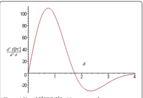
are shown in Figure 4, in which a plot of@2_{E TC½ =@}2_δis shown where the second derivative is greater than zero in the interval 0≤δ≤1:795. It implies thatE½TCis a con-vex function, and the local minimum becomes the global minimum in the specified interval.

The sensitivity of the optimal specification limit to the changes in the mean and standard deviation are shown in Tables 1 and 2, respectively. It can be observed that δgradually decreases asσincreases.

The optimal USL and LSL are 50.8% and 48.8%, re-spectively. When σ = 2.0, E L y½ ð Þ becomes larger since an increase in the key factor's choice implies a lower outgoing TT process quality.

E C½ R is dependent only on δ, and therefore, the

low-est value of E C½ R is obtained when δ = 2.23, and the

highest value is obtained whenδ = 1.40. In other words,

E C½ R is higher for lower values ofδand vice versa.

Table 1 shows that E C½ M depends on δ and σ and is

the lowest when σ is between 1.7 and 1.8. The effect of μτ

j j(i.e., process bias) onδis shown in Table 2. Finally, Table 3 shows the effect of½CM, E C½ R ,E L y½ ð Þ,

andE½TCto the changes inδandσ.

Results give an idea of the optimal choice for the key factor in the quality analysis for one, the number of in-vention disclosures, of the set of the quality indexes of TT process.

Conclusions

Managers, TT operators, and R&D managers are often faced with the problem of determining the optimal choice of key factor in the tolerance process evaluation regarding the quality of the technology transfer process.

This paper showed how the costs related to this choice are quantified and integrated and also showed how the Lambert W function is incorporated into this choice optimization problem by deriving a closed-form solu-tion. This proposed model and solution may be appeal-ing to operators since the Lambert function is found in a number of standard optimization softwares.

Results are presented, in this first paper, in terms of the number of invention disclosures as one of the in-dexes of a TT process.

Table 2 Effect ofδ*on |μ−τ|

μ(%) μ−τ σ β* E[CM] E[CR] E[L(y)] E[TC]

49.0 1.0 1.0 2.00 99.60 22.42 169.59 291.61

49.1 0.9 1.0 2.05 99.59 20.01 153.82 273.42

49.2 0.8 1.0 2.09 99.58 18.08 139.40 257.06

49.3 0.7 1.0 2.13 99.57 16.54 126.47 242.58

49.4 0.6 1.0 2.16 99.57 15.31 115.12 230.00

49.5 0.5 1.0 2.19 99.56 14.34 105.42 219.32

49.6 0.4 1.0 2.21 99.56 13.60 97.42 210.58

49.7 0.3 1.0 2.22 99.56 13.05 91.16 203.77

49.8 0.2 1.0 2.23 99.55 12.67 86.67 198.89

49.9 0.1 1.0 2.24 99.55 12.45 83.97 195.97

50.0 0.0 1.0 2.24 99.55 12.37 83.06 194.98

Figure 4Plot of∂2_E[TC]/∂2_{δwith respect toδ}

Table 1 Effect ofσonδ*

σ μ(%) μ−τ β* E[CM] E[CR] E[L(y)] E[TC]

1.0 49.8 0.2 2.23 99.55 12.67 86.67 198.89

1.1 49.8 0.2 2.19 99.52 14.32 105.44 219.28

1.2 49.8 0.2 2.13 99.49 16.39 125.65 241.53

1.3 49.8 0.2 2.07 99.46 19.00 147.14 265.60

1.4 49.8 0.2 2.01 99.44 22.32 169.69 291.45

1.5 49.8 0.2 1.93 99.42 26.58 193.00 319.00

1.6 49.8 0.2 1.85 99.41 32.09 216.65 348.15

1.7 49.8 0.2 1.76 99.40 39.31 240.05 378.76

1.8 49.8 0.2 1.65 99.40 48.93 262.32 410.65

1.9 49.8 0.2 1.54 99.42 61.95 282.18 443.55

2.0 49.8 0.2 1.40 99.44 79.97 297.60 477.01

Table 3 Relationship between costs andδ

δ(%) σ μ μ−τ E[CM] E[CR] E[L(y)] E[TC]

1.0 1.0 49.8 0.2 99.80 158.61 22.62 281.03

1.2 1.1 49.8 0.2 99.76 115.01 33.47 248.24

1.4 1.2 49.8 0.2 99.72 80.70 45.29 225.71

1.6 1.3 49.8 0.2 99.68 54.73 57.12 211.53

1.8 1.4 49.8 0.2 99.64 35.86 68.12 203.62

2.0 1.5 49.8 0.2 99.60 22.68 77.69 199.97

2.2 1.6 49.8 0.2 99.56 13.83 85.51 198.90

2.4 1.7 49.8 0.2 99.52 8.13 91.56 199.21

2.6 1.8 49.8 0.2 99.48 4.59 95.98 200.05

2.8 1.9 49.8 0.2 99.44 2.48 99.05 200.97

3.0 2.0 49.8 0.2 99.40 1.28 101.08 201.76

Appendix 1

First, we consider the indefinite integral of the integrand

z

ð Þdz. Following the definition of a standard normal ran-dom variable, the integral can be written as follows:

Z

zφð Þz dz¼ 1ffiffiffiffiffiffi

2π

p Z zez2=2dz

Substituting u into z2_{, it follows that du¼2zdz and}

zdz¼du=2 . Thus, the integral can now be written as follows:

Z

zφð Þz dz¼ 1

2pffiffiffiffiffiffi2π Z

eu=2du

As Reu=2_{¼ e}u=2 _{, we get} R_{zφð Þz dz¼} 1

2pffiffiffiffi2π R

eμ=2_du¼ 1ffiffiffiffi 2π

p _eu=2_{¼ φð Þz .}

Next, we consider the indefinite integral of z2φð Þz dz. This integration can be performed using the formula for the method of integration by parts given as follows:

Z

uvdx¼v Z

du dx

Z du dx Z

vdx

dx

If z2_{φð Þz dz is separated into two parts, namely, z and}

z

ð Þ, then the integration by parts formula can be applied as follows:

Z

z2φð Þz dz¼ Z

z zð φð Þz Þdz

¼z Z

zφð Þz dz Z

φð Þz dz

¼zφð Þ z Φð Þz

Appendix 2

Lemma 1. Suppose χ2R1 and the mapping η:χ!R be η¼χeχ, then the solution for χ is given by ¼

LambertWð Þη.

Proposition 1.Ifη₂¼ðχþη₁Þeχ, whereη₁andη₂are not functions ofχ, thenχ¼LambertWðη₂eη1Þ η

1.

Proof.The proposition can be proven using Lemma 1 starting from Equation 27 given by the following:

η2¼ðχþη1Þeχ ð27Þ

Lettingχþη₁¼ψ, Equation 27 becomes the following:

η2¼ψeψ

η1 ð₂₈Þ

To convert Equation 28 to the standard formη¼χeχ, we first modify Equation 28 as follows:

η2eη1¼ψeψη1 ð29Þ

Next, substituting η₂eη1¼ω _{into the right-hand side,}

we obtain the standard form as ω¼ψeψη1. Now,

recal-ling Lemma 1,ψcan be given as follows:

ψ¼LambertWð Þω ð30Þ

Therefore, the solution for χ can be obtained as ¼

LambertWðη₂eη1Þ η

1.

Proposition 2.Ifη₄¼η₁ðχþη₂Þeη3χ, whereη

1,η2,η3,

andη₄are not functions ofχ, then

χ¼ LambertW η3η4eη2η3=η1

η3

η2

1=2

Proof.In order to prove Proposition 2 using Lemma 1, we first consider this equation:

η4¼η1ðχþη2Þeη3χ ð31Þ

Multiplying both sides with η3/η1, Equation 31 becomes the following:

η3η4 η1

¼η3ðχþη2Þeη3χ ð32Þ

Letting ψ¼η₃ðχþη₂Þ, Equation 32 can be written as follows:

η3η4eη2η3 η1

¼ψeψ1 ð₃₃Þ

Further, substituting η₃η₄eη2η3=η

1¼ω, Equation 33 is now in the standard formη¼χeχ

ψ¼LambertWð Þω ð34Þ

Replacing ω¼η₃η₄eη2η3=η

1 back into Equation 34, the standard form in Equation 34 can be written as follows:

ψ¼LambertW η3η4e

η2η4

η1

ð35Þ

Equation 35 can be expanded to express the solution in terms of χ by substituting ψ with η₃ðχþη₂Þ. Thus, the solution forχis given as follows:

χ¼ LambertW η3η4eη2η3=η1

η3

η2

1=2

Competing interests

The author declares that he has no competing interests.

Authors’information

SDF has a Ph.D. in Electrical Engineering. He is the chief of the Technology Transfer Office of School of Sciences and Technologies of the University Federico II of Naples, and he is the adviser of TT - Technology Transfer Magazine and he is the AICTT president of the Italian Association for Promotion of Culture of Technology Transfer.

References

Avriel, M., Diewert, W. E., Schaible, S., & Zang, I. (1988).Generalized Concavity (Mathematical Concepts and Methods in Science and Engineering(Vol. 36). New York: Plenum Press.

Bazaraa, M. S., & Shetty, C. M. (1993).Nonlinear Programming. New York: Wiley. Chase, K. W., Greenwood, W. H., Loosli, B. G., & Haughlund, L. F. (1990). Least-cost

tolerances allocation for mechanical assemblies with automated process selection.Manuf Rev, 3, 49–59.

Corless, R. M., Gonnet, G. H., Hare, D. E. G., Jeffrey, D. J., & Knuth, D. E. (1996). On the Lambert W function.Advances in Computational Mathematics, 5, 329–359. Fathi, Y. (1990). Producer–consumer tolerances.Journal of Quality Technology, 22,

138–145.

Hulsebeck, M., Lehmann, E. E., & Starnecker, A. (2011). Performance of technology transfer offices in Germany.The Journal of Technology Transfer. doi:10.1007/ s10961-011-9243-6.

Jeang, A. (1997). An approach of tolerance design for quality improvement and cost reduction.International Journal of Production Research, 35, 1193–1211. Jeang, A. (1999). Robust tolerance design by response surface methodology.

International Journal of Production Research, 37, 3275–3288.

Kapur, K. C. (1988). An approach for development of specifications for quality improvement.Quality Engineering, 1, 63–77.

Keller, R. T., & Chinta, R. R. (1990). International technology transfer: strategies for success.The Academy of Management Executive, 4(2), 33–43.

Kim, Y. J., & Cho, B. R. (1999). Economic integration of design optimization.

Quality Engineering, 12, 591–597.

Kim, Y. J., & Cho, B. R. (2000). The use of response surface designs in the selection of optimum tolerance allocation.Quality Engineering, 13, 35–42.

Phillips, M. D., & Cho, B. R. (1999). An empirical approach to designing product specifications: a case study.Quality Engineering, 11, 91–100.

Quazi, H. A. (1998). Application of TQM principles in the International Technology Transfer process of industrial production plants: a conceptual framework.

British Journal of Management, 9(4), 289–300.

Reisman, A. (2005). Transfer of technologies: a cross taxonomy.International Journal of Management Science, 33, 189–202.

Roberts, A. W., & Varberg, D. E. (1973).Convex Functions. New York: Academic. Robinson, R. D. (1988).The International Transfer of Technology: Theory, Issues, and

practice. Pensacola: Ballinger Publishing.

Sarina, M. N., Rushami, Z. Y., & Fariza, H. (2009). Quality practices as a moderator in technology transfer performance.Int J Bus Manag, 4(7), 96–105. Taguchi, G., & Wu, Y. (1980).Introduction to Off-line Quality Control. Nagoya, Japan:

Central Japan Quality Control Association.

Taguchi, G. (1986).Introduction to Quality Engineering: Designing Quality into Products and Processes.: Asian Productivity Organization/American Supplier Institute.

Taguchi, G. (1993).Taguchi on Robust Technology Development: Bringing Quality Engineering Upstream. New York: ASME Press.

Tang, K. (1988). Economic design of product specifications for a complete inspection plan.International Journal of Production Research, 26, 203–217. Tang, K. (1991). Design of multi-stage screening procedures for a serial

production system.European Journal of Operational Research, 52, 280–290. Tang, K., & Tang, J. (1989). Design of product specifications for multi-characteristic

inspection.Management Science, 35, 743–756.

Tang, K., & Tang, J. (1994). Design of screening procedures: a review.Journal of Quality Technology, 26, 209–226.

doi:10.1186/2192-5372-1-6

Cite this article as:De Falco:Is it possible to control and optimize technology transfer process?.Journal of Innovation and Entrepreneurship 20121:6.

Submit your manuscript to a

journal and benefi t from:

7Convenient online submission 7Rigorous peer review

7Immediate publication on acceptance 7Open access: articles freely available online 7High visibility within the fi eld

7Retaining the copyright to your article

Submit your next manuscript at 7 springeropen.com

Received: 10 April 2012 Accepted: 8 August 2012 Published: 8 August 2012