O R I G I N A L A R T I C L E
Open Access
Shipping Optimisation Systems (SOS):
tramp optimisation perspective
Said El Noshokaty
Correspondence:
El Esteshary Information Systems (EIS), 637 Horreya Avenue, Genaklis, Alexandria 21411, Egypt
Abstract
This research paper is to announce a new policy to all systems which are sensitive to time. In tramp cargo transportation, as an example, the current policy is to select for each ship the cargo mix which contributes more to a gross-profit objective, assuming deterministic cargo transport demand. Since tramp cargo transportation is sensitive to time, where time varies considerably from one alternative ship voyage to another. The new policy considers this objective less profitable than gross-profit-per-day objective, assuming both deterministic and stochastic cargo transport demand. To introduce this new policy, SOS; a suite of decision support systems, is developed to optimise tramp shipping using a stochastic gross-profit-per-day objective. For operational purposes, SOS selects the most profitable cargo mix. This mix is selected because of the higher gross profit it is expected to yield and the less number of days it takes to generate such profit. For long-term planning purposes, SOS uses the optimal gross profit of each ship voyage, created by the system, to allocate fleet units to cargo trade areas, specifying their frequency of calls to maximise fleet annual gross profit. A useful application of this fleet allocation is that the allocated frequency of calls may be considered as
representing the demand on services of utilities of ports, canals, and straits, and may be used to assess the competitiveness of these utilities. Utility and logistics planner, via sensitivity and what-if analysis, can determine whether calling at a utility of a trade area is sensitive to changes made to utility dues and staying time, cargo quantities and freight rates, cargo handling rates and charges, and ship speed and fuel consumption. For appraising purposes, SOS includes new ships in the allocation process, in
competition with old ones, to find the share each new ship adds to total gross profit each year. SOS then applies the Net Present Value formula to gross profit of each new ship, along with other cash flow and cost of investment. SOS similar systems may be tailored for other means of cargo transport; namely cargo airplanes, trains, and trucks. The impact of SOS on any logistics and supply chain system is that it maintains the shortest possible transportation time owners of transport units can afford. Case studies are brought to demonstrate research findings.
Keywords:Optimal cargo mix, Transportation scheduling, Transportation routing, Transportation allocation, Transportation appraisal
Introduction
If compared to other businesses, cargo transportation in tramp mode has three dis-tinctive characteristics. The first characteristic is that itsproduction cycle(ship voyage) passes through different economic systems which cause uncertainty and create un-structured decision situation (Fields and Shingles 2016). In an unun-structured decision
situation, solution steps are usually not known beforehand. The second characteristic is that production time(voyage time) varies considerably from one alternativeproduction cycleto another. The production cycleis said to be time-sensitive because of this vari-ation in time. The varivari-ation is mainly caused by the alternative cargo mixes available for transport in competition with other ships, the alternative shipping routes the ship may follow towards the same cargo mix, and the alternative ship speeds at which the ship may sail. In comparison, the production cycle in liner shipping is not sensitive to time since production time is fixed where the ship sails per a predetermined itinerary (see El Noshokaty 2013). Likewise, crop harvesting in agriculture, car manufacturing and assembly lines in industry, and road paving in construction are all not time-sensitive. Time-sensitivity is known to the ship owner when he hires his ship as a time charter for a better hire per-day, main while he ignores it when he does not hire his ship as a voyage charter for a better gross profit per day (Time Charter Equivalent rate in voyage charter is not the gross profit per day as been defined in this paper). How-ever, the ship owner shows awareness of time sensitivity when he puts in the voyage charter party a clause specifying a minimum cargo loading and discharging rate. His intention is to minimise voyage time. This action influences few cost and revenue items plus cargo handling days, while a gross-profit-per-day objective influences all cost and revenue items plus all voyage days, including sailing and waiting days. The gross-profit-per-day objective is more described hereinafter. The third characteristic is that trans-portation unit calls at a variable number of stops and follows many calling sequences among these stops. In other words, a transportation unit does not operate on a pub-lished schedule but serves different stops in response to tenders of cargo. It runs like a taxi cab in private transport if compared to a bus in public transport. This mode of op-eration requires, in model terminology, many variables and constraints which in turn requires the use of mathematical models (Christiansen and Fagerholt 2014).
mentioned earlier. In contrast, the current practice of ship owners is to choose cargo A with a Time Charter Eqivalent rate of $ 10,000. The third problem is the need to ex-plore massive alternative solutions before reaching the optimal solution. Fortunately, Operations Research (OR) techniques provide such solution methodology. The impact of the optimal solution provided by OR on any logistics and supply chain system is that it maintains the shortest possible transportation time owners of transport units can af-ford. The challenge in using OR models is in including all the necessary parameters and business rules that represent a real cargo transport problem. And, because some of these parameters are fixed, they need to be checked for validity. Also, OR models have to be incorporated within a decision support system in order to allow non-OR users to deliver model parameters, and to run and interact with these models.
the new ships along with the old ones in the allocation plan to find the share each new ship adds to total gross profit each year. SOS uses the new ship gross profit, along with other cash flow and cost of investment, to calculate the net present value of this new ship.
In the following section, current research papers are discussed to prove that the above-mentioned comments are true, and to see what possible contribution that could be made by this research paper to avoid these comments. A problem statement is for-mulated side by side along with the review of the literature.
Problem statement and review of the literature in tramp shipping optimisation
The term ‘tramp shipping optimisation’ refers to the use of OR to maximise the rev-enue or minimise the cost of a tramp shipping problem, subject to the limited shipping resources. One such tramp shipping problem exists when there are some ships and some cargoes and it is required to find out the cargo mix assigned to each ship voyage which maximises total gross profit per day for all ships, subject to ship capacity and cargo time window (lay can). Name this problem area‘optimisation of ship voyage’. To give more details on this area, consider the following facts. Unlike‘optimisation in liner shipping’, both ports of call and port calling sequence are here assumed optional. Char-ter party, signed by the ship owner and the charChar-terer, usually specifies Char-terms and clauses to be followed by both parties. Non-demise voyage charter parties are assumed here. Terms generally include the following items: calling ports, calling sequence, cargo freight, cargo time window (lay can), allowable cargo handling time (lay days), dispatch count if actual days are less than lay days, and demurrage count if more. Loading and discharging lay days may be considered in reversible or irreversible manner. If revers-ible, lay days are specified for loading and discharging collectively. If irreversrevers-ible, lay days are specified for loading and discharging separately. The gross terms of voyage charter party are here assumed unless otherwise specified. Before cargoes are being fixed by the ship owner,‘optimisation of ship voyage’helps in proposing a voyage plan suggesting an optimal cargo mix for each ship. This mix maximises the sum of voyage gross profit per day for all ships, subject to ship capacity, cargo lay can, and other voy-age charter party terms. In the cargo mix selection, the random nature of sea transport demand has to be considered.
cost. The review of these research papers is reported in the follows items. The first is that their research model is most useful for bulk carriers since it assumes only one cargo to be loaded at a time. The second is that the problem known in the literature as the‘fixed-charge problem’is not addressed. In this problem, fixed charges; such as port dues, are to be paid no matter how many cargoes ship selects in each port. The third is that the objective does not consider the time taken to earn revenues. In tramp shipping, revenue or gross profit per day is a common objective.
Bauch et al. (1998) and Bremer and Perakis (1992a, 1992b) have put emphasis on ap-plication and implementation using an OR model not much different than that of Appelgren. The authors have captured raw data about cargoes, ships, ports, and dis-tances and use it to generate all possible schedules for each ship. Each schedule identi-fies several cargoes to be transported, arranged and put in a predetermined sequence. Data pertaining to these schedules is input to an integer programming package as pack-age parameters. The packpack-age was run to select the set of schedules that gives an opti-mal solution. The same review mentioned about Appelgren applies also here, plus the fact that the generation of all possible schedules is not guaranteed.
Fagerholt (2001) has developed an optimisation model for tramp shipping, where cargo time window (lay can) may be violated to a certain extent with a penalty cost in return. That is why cargo time window was given the name soft time window,and pen-alty cost was given the name inconvenience cost. The model designs a predetermined set of schedules for each ship to follow. In each schedule, there is a predetermined route with cargo pick-up and delivery nodes along with soft time window for each node and a predetermined ship speed on each sailing leg. The model objective is to find the schedule for each ship which minimises total operating and penalty cost. The review of this model is reported in the follows items. The first is that the number of schedules of each ship is too small to represent all candidate schedules. The second is that even if the number of schedules is large enough, the way the schedule is designed does not generate a right mix between low and high-cost schedules. The right mix has to be the one that leads to a globally optimal solution. The third is that the model does not use gross profit or gross profit per day as a criterion for selecting optimal schedules, which limits the use of the model to only the industrial mode of transport. The fourth is that transport demand is assumed fixed.
Fagerholt (2004) has also developed a computer-based decision support system for fleet scheduling based on heuristic algorithms. Fagerholt et al. (2010) have presented a decision support methodology for strategic planning in tramp and industrial shipping. The proposed methodology combines simulation and optimisation, where a Monte Carlo simulation framework is built around an optimisation-based decision support system for short-term routing and scheduling. Although these research papers have de-veloped algorithms which are flexible, allow interactive user interface, and save time, their exact optimal solution is not guaranteed.
have similar capacity. The third is that full ship loads are assumed. The fourth is that consecutive loads are not allowed because the planning period is too short to accom-modate more than one ship load. The fifth is that the model does not use gross profit or gross profit per day as a criterion for selecting optimal schedules. The sixth is that transport demand is assumed fixed. Kim and Loe (1997) have developed a decision sup-port system for ship scheduling in industrial bulk trade. The solution method is similar to what is given by Brown et al. (1987).
Lin and Liu (2011) have considered the ship routing problem of tramp shipping and proposed a combined mathematical model that simultaneously takes into account the ship allocation, freight assignment and ship routing problems. To solve this problem, they have developed an innovative genetic algorithm. The review of this model is re-ported in the follows items. The first is that multi-commodity concept considered by this model is reduced to maximum one primary cargo and one spot cargo was taken one after the other by any ship voyage. The second is that the model does not use gross profit per day as a criterion for selecting an optimal solution. The third is that transport demand is assumed fixed.
Laake and Zhang (2013) have developed a model to determine the best mix of long-term and spot cargo contracts for a given fleet. The model finds the optimal fleet size and a mix for a set of cargo contracts or a mix of both. The model assumes that trans-port demand is sufficiently large on each route. Each ship takes full loads and does not mix cargoes from different cargo contracts, which is a standard practice in the coal/ iron ore trade. The review about Lin and Liu paper applies here also.
simultaneously on board each ship. The review of the previous models is reported in the follows items. The first is that the model objective maximises voyage gross profit, while in tramp shipping the objective has to maximise gross profit per day. The second is that transport demand is assumed deterministic. In shipping, some cargoes may have random demand. The third is that the model with non-linear objective or/and con-straints call for software solutions usually less reliable and inefficient. The fourth is that the authors brought no evidence on the possibility of solving large problems when more cargoes and ships are added.
Bakkehaug et al. (2016) and Vilhelmsen et al. (2017) have developed a similar model to schedule the voyages of a fleet of ships considering a minimum time spread between some voyages. The former has used the Adaptive Large Neighborhood Search (ALNS) heuristic to solve the problem, while the latter has used a Decomposition approach with Dynamic Programming algorithm for column generation. Their model focuses on the time spread between voyages in response to a charter party clause which requires the voyages to be
‘fairly evenly spread’. This requires the voyage to become the model decision variable with a predetermined route and full-load cargo to be transported in each voyage. This might be true for some contracted cargoes, but not true otherwise. Therefore, these two research papers cannot stand as‘optimisation of ship voyage’research area as defined earlier.
There are three additional review items that cut across all research papers mentioned so far which can be summarised as follows:
a) Model parameters are not verified for validity, using sensitivity and what-if analysis, especially for cargo quantity and freight, cargo handling rate and charges, and ship speed and fuel consumption.
b) Many shipping elements and charter party terms and clauses are not considered. Twenty of such elements and terms are shown inSOS voyager optimisation model. c) Models need OR skills to use them. In shipping, most users lack such skills.
Another problem in tramp shipping also exists when there are some ships and some trade areas, and it is required to allocate these ships to these trade areas, in an attempt to identify which trade area best fits the characteristics of each ship. The objective would be to maximise fleet gross profit, subject to available cargo demand in each trade area and yearly working days for each ship. Name this research area ‘optimisation of ship allocation’. It goes without saying that this area is of a tactical planning nature, compared to the previous research area which is of an operational planning nature. On
‘optimisation of ship allocation’research area, the following research efforts were cited. Tsilingiris (2005) addressed the problem of optimal allocation of ships to shipping lines in liner shipping, which is applicable also to tramp shipping. Two models, published by Jaramillo and Perakis (1991a, 1991b) and Powell and Perakis (1997), were used by Tsi-lingiris to allocate numbers of ship types to the routes developed in his model. The ob-jective is to find the optimal allocation of ships to routes that minimises total operating and lay-up cost. There are two review items on these research papers. The first is that voyage revenue is assumed fixed, either because cargo mixes are not considered or cargo transport demand is assumed deterministic. This means that revenue is supposed to have no effect on ship voyage and allocation of ships to lines, which is not true. The second is that allocation is done to the number of ships of each ship type, rather than the number of voyages of each ship. Allocation by the number of ships does not permit a ship to work on different lines.
Christiansen et al. (2007) and Fagerholt and Lindstad (2000) discussed an allocation model to allocate voyages of heterogeneous ships to shipping routes. The objective is to find the optimal allocation of ships to routes that minimises total operating cost plus fixed cost. There are three review items on these research papers. The first is that voyage rev-enue is not included in the model objective, ignoring the effect of revrev-enue on the alloca-tion. The second is that ship fixed cost is associated with the use of the ship. If the ship is laid up (not used), its fixed cost is going to disappear from the objective function. The third is that the model puts a maximum number of voyages for each ship in the planning period. This number is put on the total number of voyages completed by the ship on all routes. Since voyage days are not equal among routes, this number is difficult to calculate. Vilhelmsen et al. (2013, 2015) explore the tank allocation problem in bulk shipping and devise a heuristic solution method that can find feasible cargo allocations. The method relies on a greedy construction heuristic for finding feasible allocations and local search for improving initially constructed allocations.
which implies both the scheduling and routing processes, cares for the alternative pro-duction cycles of the same ship caused by the alternative cargo mixes available for transport. It is given to cargo mix selection made in a short-term plan, say 3 to 4 months at most (as in any ship voyage), whereas the name ‘optimisation of ship allo-cation’, which implies the routing process only, cares for the alternative production cy-cles caused by the alternative trade areas available for service. It is given to allocating ships to trade areas in a long-term plan, say 1 year at least (as in budgeting).‘ Optimisa-tion of ship voyage’ for a long-term plan is not advised in this research paper, where scheduling process is practically impossible to realise. The reason is that short-term plans, overlapped in a dynamic way, cares for varying and detailed shipping elements and rules. Long term plans, like macro plans, care for aggregated elements and rules. These plans enable handling of many ships and cargoes, which short term plans with detailed elements and rules cannot accommodate without too many complications. And if accommodated, optimisation cannot be done in a reasonable amount of time.
The third problem in tramp shipping also exists when there is a need to appraise a new ship; a ship to be built, purchased, or chartered-in. Name this research area‘new ship ap-praisal’. This area is of a strategic nature if compared to the above-mentioned two areas.
The reason why the above three research areas were selected among other research areas is that they are totally connected in a series of strategic, tactical, and operational planning. They aim at a common goal of not only improving the return on investment in a cargo transporta-tion domain but also improving the logistics and supply chain systems this domain is part of. Improving ship voyage objective, the way mentioned above cannot contribute positively to this common goal unless ships are allocated profitably among trade areas. Also, existing ships cannot be allocated among trade areas without taking new ships, if any, into account.
The third section discusses‘optimisation of ship voyage’, the forth section discusses‘ op-timisation of ship allocation’, and the fifth section discusses‘new ship appraisal’, along with the contribution brought in each of these research areas. The sixth section concludes the contribution made in this research paper and suggestions for future research work.
SOS Voyager optimisation
The first subsection describes the SOS Voyager optimisation model. In the second sub-section, sensitivity analysis and what-if analysis are used to validate the model. In the third subsection, a case study is presented to show the application of the model.
SOS Voyager optimisation model
This OR model aims at finding the optimal cargo mix to be assigned to each ship voyage. Its objective is to maximise the gross profit per day earned by all ships’voyages completed during a certain planning period. A simplified version of this model is displayed in Appen-dix 1. The model contains 11 basic elements and rules found in any tramp shipping prob-lem. An extended model has also been developed to include the following 9 additional shipping elements and charter party clauses (refer to SOS, 2018 for details):
specified. If the ship name is specified, booked cargo is assigned to this ship. If the ship name is not specified, booked cargo is assigned to the ship contributing more to gross profit per day.
c) Lightening of shipload via SUMED pipeline in Suez Canal.
d) Lightening of shipload via‘daughter-ship arrangement’in Suez Canal or Panama Canal.
e) Additional charter party terms such as specifying multiple ships and cargoes in one charter party, with freight specified for each cargo or lump sum freight for all cargoes.
f ) Time charter to be taken as an alternative venture to voyage charter. g) Deadweights other than winter deadweight; namely summer and tropical
deadweights.
h) Weather condition as an element affecting ship speed.
i) Different open and close ports and dates are specified for each ship.
Appendix 1 contains the model objective function, flow constraints, capacity con-straints, time concon-straints, and non-negativity and integrality constraints. The objective function is expressed in total voyage gross profit per day for all ships. The flow con-straints connect selected cargo transport links of each ship from voyage beginning to voyage end. They also ensure the flow of at most one transport link towards each cargo. The capacity constraints ensure the ship capacity; expressed in weight, volume, or units, is not violated by the cargo mix selected in each transport link. They also decide whether the ship has to be in a laden or a ballast position when sailing the transport link, and decide whether to pass or bypass the canals and straits. The time constraints ensure the time window allowed for loading or discharging of each cargo is not violated by the time spent in ports and sailing towards the cargo. They also calculate the ship waiting time spent before the opening time of each cargo time window. Also, they en-sure the total voyage allowable time is not violated by the actual time. The non-negativity constraints ensure the model variables do not go negative. The integrality constraints turn the variables, dedicated for the transverse of transport links and chartering-in, to yes-or-no decisions. A chance-constrained (stochastic) version of the model is described at the end of the Appendix. The reason for formulating the model as chance-constrained is that it consumes a smaller number of variables if compared to Dual-Stage or Multi-Stage Stochastic models, which are likely to be beyond practicality for most real linear programming applications.
The contribution made in this model is in the formulation of the objective function so that it represents a stochastic gross profit per day objective, in addition to the for-mulation of all possible shipping elements and charter party clauses.
SOS Voyager sensitivity and what-if analysis
solution. This permits the user to validate the model in capturing and describing the original problem mentioned in Problem Statement and Review of the Literature in Tramp Shipping Optimisation. In the sensitivity analysis, series of changes are given to SOS Voyager to see how far these changes are effective. In what-if analysis, a single change, in an interactive mode, is input to SOS Voyager to see the effect of this change on the objective function. Speed sensitivity or what-if analysis may be applied to all transport links collectively, or to selective transport links separately. Clicking menu op-tions is all that is needed to perform optimisation, sensitivity, and what-if analysis.
Case study on voyage optimisation
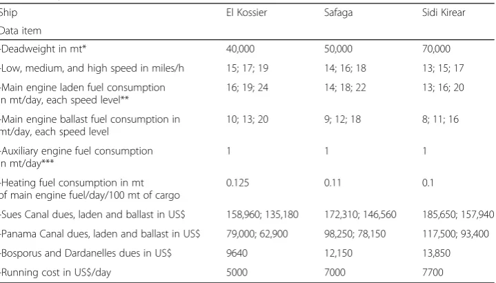
This case demonstrates the operation of a shipping company, where names and data el-ements were used to serve the purpose of this research and preserve its confidentiality. It applies the model mentioned in the first subsection and the sensitivity and what-if analysis referred to in the second subsection. It demonstrates the case where using a gross profit objective, with deterministic transport demand is considerably less profit-able than using a gross-profit-per-day objective, with stochastic transport demand. El Kosseir, Safaga, and Sidi Kirear are three oil tankers owned by Elesteshary Shipping Company (ESC). In the last quarter of the year 2017, these tankers are planning to compete in carrying ten crude oil cargoes. Three of these cargoes are to be transported from Kuwait to the USA, another three from Ukraine to China, and four from Venezuela to Latvia. Data on tankers, ports, and cargoes can be displayed and extracted using‘Data Entry Main Menu’displayed by SOS Data. Relevant data on ships is shown in Table 1. For El Kosseir and Sidi Kirear, the open port is Alexandria, Egypt. For Safaga, the open port is Odessa. For all ships, the close port is last port of call, the open date is 1/10/2017 (dd/mm/yyyy is the date format), the close date is 31/12/2017, the voyage fixed cost is $1000, and the fixed time is 0.3 days. Relevant data on the port is shown in Table 2. Before the open date, ten crude oil cargoes are identified, of which
Table 1Ship data
Ship El Kossier Safaga Sidi Kirear
Data item
-Deadweight in mt* 40,000 50,000 70,000
-Low, medium, and high speed in miles/h 15; 17; 19 14; 16; 18 13; 15; 17
-Main engine laden fuel consumption in mt/day, each speed level**
16; 19; 24 14; 18; 22 13; 16; 20
-Main engine ballast fuel consumption in mt/day, each speed level
10; 13; 20 9; 12; 18 8; 11; 16
-Auxiliary engine fuel consumption in mt/day***
1 1 1
-Heating fuel consumption in mt of main engine fuel/day/100 mt of cargo
0.125 0.11 0.1
-Sues Canal dues, laden and ballast in US$ 158,960; 135,180 172,310; 146,560 185,650; 157,940
-Panama Canal dues, laden and ballast in US$ 79,000; 62,900 98,250; 78,150 117,500; 93,400
-Bosporus and Dardanelles dues in US$ 9640 12,150 13,850
-Running cost in US$/day 5000 7000 7700
* mt = metric ton
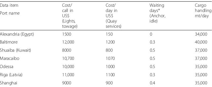
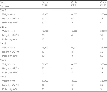
seven cargoes have confirmed (offered) quantity and freight and three unconfirmed car-goes (not yet offered). Relevant data on cargo is shown in Table 3. For the three uncon-firmed cargoes, ship owner anticipates probabilities for five classes of quantity and freight for each cargo. Ship owner also stipulates, by a least probability, to be able to transport a quantity of each cargo within its transport demand. Additional data of un-confirmed cargo is shown in Table 4. From the seven un-confirmed cargoes, ship owner needs to know what optimal (best) cargo mix to select for each ship to fix it, taking into account the three unconfirmed cargoes which might be confirmed later on. During ini-tial selection, ship speed is assumed to be at its lowest level. After the iniini-tial selection, ship owner needs to have answers to the following questions. What if the unconfirmed cargoes are all disregarded? What is the best optimisation model to use? Can further negotiation with shippers of the seven confirmed cargoes improve voyage gross profit per day? If yes, what cargo is best negotiable and what is the best quantity agree-able to both sides? If the ship speeds up to save some sailing days, do these days allow
Table 2Port data
Data item Cost/
call in US$ (Lights, towage)
Cost/ day in US$ (Quay services)
Waiting days* (Anchor, idle)
Cargo handling mt/day Port name
Alexandria (Egypt) 1500 150 0 34,000
Baltimore 12,000 1200 0.3 40,000
Shuaiba (Kuwait) 8000 800 0.5 37,000
Maracaibo 10,700 1070 0.5 37,000
Odessa 10,000 1000 0.5 35,000
Riga (Latvia) 11,000 1100 0.3 35,000
Shanghai 9000 900 0.4 35,000
* Port waiting days are classified as‘force majeure’and hence are not part of any demurrage or dispatch time counts
Table 3Cargo data
Data item Shipping
event
Load port Load Laycan
Discharge port
Discharge Laycan
Weight in mt
Freight In US$/ mt*** Cargo**
Crude Oil 1 Offered Shuaiba 1-10/10 Baltimore 1-10/11 40,000 50
Crude Oil 2 Offered Shuaiba 20-27/10 Baltimore 20-27/11 60,000 60
Crude Oil 3 Offered Odessa 5-15/10 Shanghai 5-15/11 35,000 40
Crude Oil 4 Offered Odessa 3-16/11 Shanghai 3-16/12 40,000 50
Crude Oil 5 Offered Maracaibo 5-15/12 Riga 20-30/12 30,000 30
Crude Oil 6 Offered Maracaibo 20-30/11 Riga 10-25/12 45,000 35
Crude Oil 7 Offered Maracaibo 1-10/12 Riga 20-30/12 40,000 40
Crude Oil 8 Unconfirmed Shuaiba 1-31/10 Baltimore 1-30/11 uc* uc
Crude Oil 9 Unconfirmed Odessa 1-30/11 Shanghai 1-31/12 uc uc
Crude Oil 10 Unconfirmed Maracaibo 1-30/11 Riga 1-30/11 uc uc
* uc = unconfirmed quantity or freight
** All cargoes require heating, at ship owner’s account. Crude Oil 1, 2, and 8 are transported directly (10,147 miles with 1.5 days waiting) or via Suez Canal (8602 miles with 2 days waiting), Crude Oil 3, 4, and 9 are transported directly (14,169 miles with 1 day waiting) or via Suez Canal (8264 miles with 1 day waiting), and Crude Oil 5, 6, 7, and 10 are transported only directly (5274 miles with 0.5 day waiting). Distance between ballast transport links may be found in any distance table (waiting days are assumed zero for these links).
the ship to meet lay can of more cargoes and therefore improve voyage gross profit per day? If yes, on what leg should the ship speeds up and sails on what speed?
At the beginning, SOS Voyager optimisation model is used to find the optimal (best) cargo mix for each ship. Data in Table 4 is turned to deterministic-equivalent quantities as shown in Table 5 (see end of Appendix 1 for details).
Although the number of cargoes is limited, Table 3 amended by Table 5 reads many alternative cargo mixes for each ship. When ‘Tramp Shipping Optimisation Main Menu’ of SOS Voyager is displayed and when ‘Optimisation and Sensitivity Analysis’ option is selected from the menu, the sensitivity analysis is reported as in Table 6. To reach the stage where Table 6 is reported, SOS Voyager, as a decision support system, must do a lot of tasks. Details of these tasks are included in Appendix 4.
The model report for high-speed shown in Table 6 is broken down into the voyage details displayed in Table 7.
Suppose now that unconfirmed cargoes: ‘Crude Oil 8’,‘Crude Oil 9’, and ‘Crude Oil 10’are discarded, the profit-per-day criterion is also discarded and gross profit objective
Table 4Unconfirmed cargo additional data
Cargo Crude
Oil 8
Crude Oil 9
Crude Oil 10 Data item
Class 1
Weight in mt 45,000 40,000 30,000
Freight in US$/mt 50 45 35
Probability in % 5 10 5
Class 2
Weight in mt 47,000 42,000 32,000
Freight in US$/mt 50 45 35
Probability in % 15 25 15
Class 3
Weight in mt 49,000 44,000 34,000
Freight in US$/mt 50 45 35
Probability in % 50 40 60
Class 4
Weight in mt 51,000 46,000 36,000
Freight in US$/mt 50 45 35
Probability in % 20 15 15
Class 5
Weight in mt 53,000 48,000 38,000
Freight in US$/mt 50 45 35
Probability in % 10 10 5
Table 5Unconfirmed cargo deterministic-equivalent quantity and freight
Cargo Data item Crude Oil 8 Crude Oil 9 Crude Oil 10
Weight in mt 51,000 42,000 36,000
Freight in US$/mt 50 45 35
is used instead (which can be handled also by SOS Voyager). Table 8 displays results of this supposed case, assuming all ships are at high speed.
Table 8 is broken down into the voyage details displayed in Table 9. The following are some analysis made upon examining Tables 6 to 9:
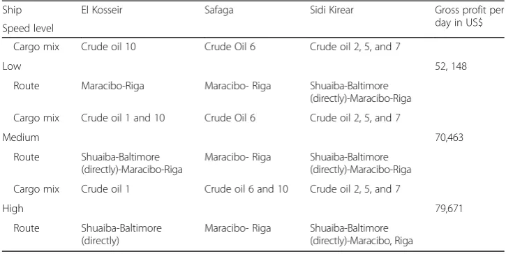
a) The number of alternative cargo mixes in the model is enormous and thus cannot be manually enumerated. It takes SOS Voyager 1 min to process the model. Hardware used is Intel i3 PC (64-bit). Software used is MS Windows 7. MS Access 2007 is used as a front-end database system, while MS SQL Server 2008 is used as a back-end database to permit data to expand and to be updated from different net-work entry points, locally and remotely. Microsoft Message Passing Interface (MS MPI) is used for parallel processing. Processes may be distributed among cores of one PC or cores of multiple PCs in a network. The 1 min was taken on one i3 PC. Using old software versions has no effect on model performance if compared to computer hardware and network facilities. SOS is designed primarily to handle a scale of up to 30 ships and 30 cargoes. Although time was not recorded for such scale, an experiment was made which may be used as a guide to estimate processing time, that is to run the model for one ship and 30 cargoes. The reason why only one ship is chosen is that the algorithm used to process the model can decompose the shipping problem into sub problems, one for each ship. Meanwhile, MS MPI can process the 30 sub-problems in parallel with each sub-problem using one pro-cessor core. It takes SOS Voyager 58 min to process the model for 1-ship-30-cargo Table 6Cargo mix, route, and gross-profit-per-day reported by the model (with gross profit per day objective) for each ship, classified by speed level
Ship El Kosseir Safaga Sidi Kirear Gross profit per
day in US$ Speed level
Cargo mix Crude oil 10 Crude Oil 6 Crude oil 2, 5, and 7
Low 52, 148
Route Maracibo-Riga Maracibo- Riga Shuaiba-Baltimore
(directly)-Maracibo-Riga
Cargo mix Crude oil 1 and 10 Crude Oil 6 Crude oil 2, 5, and 7
Medium 70,463
Route Shuaiba-Baltimore (directly)-Maracibo-Riga
Maracibo- Riga Shuaiba-Baltimore (directly)-Maracibo-Riga
Cargo mix Crude oil 1 Crude oil 6 and 10 Crude oil 2, 5, and 7
High 79,671
Route Shuaiba-Baltimore
(directly)
Maracibo- Riga Shuaiba-Baltimore (directly)-Maracibo, Riga
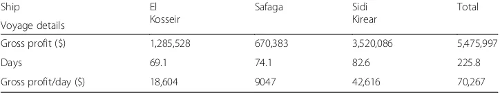
Table 7Voyage details reported by the model (with gross profit per day objective) for each ship, at high speed
Ship El
Kosseir
Safaga Sidi
Kirear
Total
Voyage details
Gross profit ($) 752,534 1,145,939 3,520,082 5,418,555
Days 34.4 75.5 82.6 192.5
scale, using the above-mentioned hardware and software. Remember that the model has a gross-profit-per-day objective which requires additional algorithms and con-tains all possible shipping elements and charter party clauses which require add-itional constraints. Add to this the fact that the 30 cargoes create an enormous number of alternative transport links which requires additional variables. These re-quirements demand considerable processing time. It goes without saying that prob-lem scale and timing rely heavily on computer hardware and network architecture, e.g. a supercomputer will dropdown processing time considerably. The software is designed carefully to handle large-scale problems. It should be noted in this respect that the 30-ship limit is put on the number of ships of the same type that could compete in carrying same cargoes in the same planning period. Likewise, the 30-cargo limit is put on the number of 30-cargoes of the same type that are available for transport on board these ships in the same planning period. To handle the case of 30 or more cargoes when computing resources are limited in speed, the user may partition the planning period, say 3 months, into smaller ones, say 1 month each. In this case, the optimal cargo mix selected for a certain ship in 1-month planning period is considered as already discharged, still loaded, or still booked for this ship in the next planning period, where planning periods may overlap. In the next plan-ning period, new cargoes may be added as being offered or not-yet-offered. The ad-vantage of this arrangement is not only to handle a smaller number of cargoes in each period but also to incorporate changing shipping elements over time. The dis-advantage is to lose a longer term planning.
b) In this case study, speed sensitivity analysis concludes that the higher speed is tried on all legs the more gross profit per day or gross profit is achieved. Higher speed enabled each ship to meet lay can dates of more profitable cargoes. One can expect better results if higher speed is tried only on legs leading to these cargoes.
Sensitivity analysis may also be tried for cargo freight and quantity, and cargo handling rate and charges. Take for now handling rate as an example. There is a chance that handling rate in Maracaibo be decreased to 17,000 mt/day due to Table 8Cargo mix, route, and gross profit reported by the model (with gross profit objective) for each ship, at high speed
Ship El Kosseir Safaga Sidi Kirear Gross profit
in US$ Speed level
Cargo mix Crude oil 1 and 4 Crude oil 3 and 6 Crude oil 2, 5, and 7
High 5,475,997
Route Shuaiba-Baltimore(directly)-Odessa-Shangahai (via Suez Canal)
Odessa -Shangahai
(via Suez Canal)-Maracibo-Riga (via Panama Canal)
Shuaiba-Baltimore (directly)-Maracibo-Riga
Table 9Voyage details reported by the model (with gross profit objective) for each ship, at high speed
Ship El
Kosseir
Safaga Sidi
Kirear
Total
Voyage details
Gross profit ($) 1,285,528 670,383 3,520,086 5,475,997
Days 69.1 74.1 82.6 225.8
pumps repeated malfunction. There is also another chance that by the time Sidi Kirear reaches Maracaibo in early December to take‘Crude Oil 5’and‘Crude Oil 7’, handling rate could possibly reach 57,000 mt per day. This may be caused by the installation of high-speed pumps. Applying handling sensitivity to the model at low-speed results the same quantities as what were reported earlier, for the two handling rates available for Sidi Kirear while loading‘Crude Oil 5’and‘Crude Oil 7’. The only difference between the two rates is that total gross profit per day decreases to $ 51,521 for 17,000 mt/day and increases to $ 52,339 for 57,000 mt/day handling rate. c) In comparison between Tables7and9, one can notice that the model can increase
gross profit per day by $ 9404 (13%) while maintaining same gross profit as that given by Table9(think of the percentage improvement in gross profit per day if the ship owner adopts the ship full-load-and-down criterion). With full confidence in probabilities shown in Tables4and5, this analysis recommends that unconfirmed
‘Crude Oil 10’suggested by Table7is better being selected instead of confirmed
‘Crude Oil 3’and‘Crude Oil 4’suggested by Table9. As perhaps noticed, if the ship operator decides on the cargo mix suggested by Table9, he will not be able to select
‘Crude Oil 10’when it is confirmed later on, losing $ 9404 gross profit per day. The previous analysis suggests also that stochastic gross profit per day is expected to be more profitable than stochastic gross profit.
d) If probability distribution cannot be identified for cargo transport demand, then the model can be used along with quantity-and-freight sensitivity analysis of unconfirmed cargoes. In this case, ship owner’s own judgment is needed to select between the alternative outcomes of sensitivity analysis. This analysis will leave gross profit criterion the last choice in selecting the optimal cargo mix. To explain, suppose ‘Crude Oil 9’ and‘Crude Oil 10’ become confirmed with quantities and freights shown in Table 5, while ‘Crude Oil 8’ is still un-confirmed with no such probability distribution as shown in Table 4. Suppose now that ship owner wants to evaluate the effect of ‘Crude Oil 8’ quantity-and-freight change on gross profit per day at low ship speed, namely at quan-tities of 35,000 mt, 45,000 mt, and 55,000 mt with freights of $ 60, $ 55, and $ 50, respectively. Applying gross profit per day objective, with quantity and freight sensitivity analysis, results the same as what is given by the model at low speed, for all quantities. In other words, the objective is not sensitive to the change in the quantity and freight of ‘Crude Oil 8’. This analysis suggests the use of stochastic gross profit per day or gross profit per day when com-pared to gross profit.
f ) The above-mentioned analysis uses sensitivity analysis. What-if analysis may also be applied after optimisation has taken place, with or without sensitivity analysis, to show the effect of only one change level in model parameter, whether the model is of voyage gross profit or gross profit per day. Cargo freight rate and quantity, cargo handling rate and charges, and ship speed and fuel consumption are examples of such parameters.
g) The above-mentioned analysis assumes all ships are owned. What if the ship owner decides to charter-in a ship as to compete in carrying‘Crude Oil 6’for example? The estimated gross profit of the chartered-in ship is $ 400,000 in 25 days with $ 1000 voyage fixed cost and 1 day voyage fixed time. Assuming ship low-speed with no sensitivity analysis applied to the model, the result would be: carry‘Crude Oil 4’ by Safaga via Sues Canal,‘Crude Oil 10’by El Kosseir directly,‘Crude Oil 2’followed by‘Crude Oil 5’and‘Crude Oil 7’by Sidi Kirear, all directly, then‘Crude Oil 6’by the chartered-in ship. Total gross profit per day would be $65,969.
h) Optimisation sessions may be repeated once again later; say next month. At that time, old offers may become fixed or loaded, not-yet-offered cargoes may become offered, and new offers and probable cargoes may be added.
The above-mentioned analysis recommends the use of stochastic gross profit per day objective and the use of gross profit per day objective plus quantity-and-freight sensi-tivity analysis of unconfirmed cargoes in case probability distribution cannot be identi-fied for cargo transport demand. The analysis does not recommend the use of gross profit objective or stochastic gross profit objective, as they are expected to give less profit per year. The key elements in the previous analysis are ‘gross profit per day ob-jective’along with‘stochastic cargo transport demand’and‘optimisation with sensitivity and what-if analysis’. Owners of tramp shipping systems or any tramp-like transport systems; namely those of cargo airplanes, trains, and trucks, are encouraged to adopt management policies that maintain these key elements.
SOS Allocator optimisation
The following subsection describes the SOS Allocation model, followed by a subsection to demonstrate a useful application of this model; a case study on port development.
SOS allocation model
The contribution made in this model is in the formulation of the objective function so that it represents a gross profit rather than mere cost items. The contribution is also in the use of gross profit generated from an integrated system like SOS Voyager, as-suming realistic cargo transport demand, deterministic or stochastic, available on each cargo trade area. In this model, each ship can work on more than one trade area and to load more than one cargo. SOS may always roll back to SOS Voyager in case its param-eters, as described in the next section, are subject to change. In this case, another SOS Allocator session is tried. It goes without saying that the more model parameters are truly representing all possible maritime logistics, the more rigorous is the demand as-sess on port services. Model validity is guaranteed by the sensitivity and what-if analysis used by the model, as described in next section.
Case study on port development
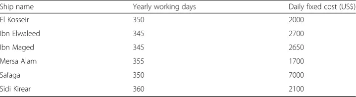
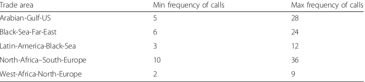
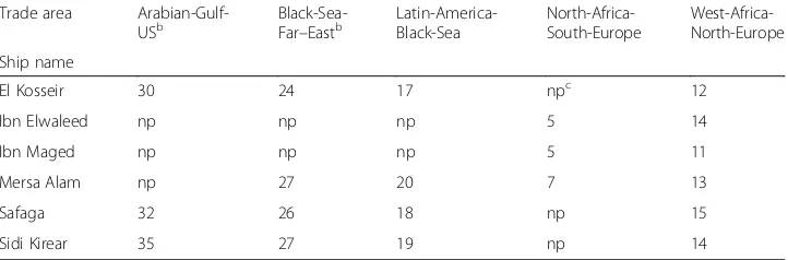
The purpose of this case is to show the application of the model mentioned in SOS Al-location model. A shipping research institute called Shipping Research Center (SRC) is now preparing a report on world port development for year 2018. To cover the oil trade part of this report, SRC decided to consult several oil shipping companies on their next year operational plan, as to size the demand on world port services for oil trade. One of these companies is called Elesteshary Shipping Company (ESC), which owns six oil tankers of types used in the marketplace. For the purpose of this research, consider this number of tankers as actually representing the oil shipping industry. To prepare the operational plan for the year 2018, ESC decided to revise the current allo-cation of ships to oil trade areas. For this purpose, ESC tried to figure out different voy-ages for each ship, one in each trade area. Cargo transport demand (quantity and freight rate) was then anticipated for a most-likely voyage most presenting each trade area. SOS Voyager was then run to calculate voyage gross profit for each ship on each trade area. Voyages failed to earn any gross profit were discarded. SOS Allocator was then run to see what ship best fits on which trade area, and the frequency of calls it best completes in this trade area. In Table 10, data required for SOS Allocator is dis-played by ship working days and daily fixed cost in the year 2018. Trade area minimum and maximum frequency of calls in the year 2018 is displayed in Table 11. The most-likely voyage gross profit in the year 2018 classified by ship and trade area is displayed in Table 12. Average voyage time in the year 2018, classified by ship and trade area, is also shown in Table 13.
To describe how data in Tables 12 and 13 is calculated, take ship El Kossier as an ex-ample when it works on Arabian-Gulf-US trade area. According to SOS Voyager, El
Table 10Ship yearly working days and daily fixed cost in 2018
Ship name Yearly working days Daily fixed cost (US$)
El Kosseir 350 2000
Ibn Elwaleed 345 2700
Ibn Maged 345 2650
Mersa Alam 355 1700
Safaga 350 7000
Kossier earned last quarter of the year 2017 a gross profit of $ 710,500 in a 30-day voy-age, where 15-knot speed is assumed and some unconfirmed cargoes are considered. This data is chosen to represent the result of El Kossier when it works on Arabian-Gulf-US trade area in the year 2018. It appears as one entry in Tables 12 or 13. So, these tables present all candidate alternatives of voyage gross profits and days for all ships in all trade areas, calculated per an anticipated cargo transport demand in each trade area. Table 10 presents the supply of ships in terms of available working days and ship daily fixed cost per the year 2018, while Table 11 presents the minimum and max-imum frequency of calls in each trade area. Data in Tables 10 and 11 is input to SOS Data (the SOS database), while SOS Voyager generates data in Tables 12 and 13.
Using SOS Allocator model, given data in Tables 12 and 13, it is required to find the optimal allocation of ships to trade areas and lay-up days of each ship satisfying data in Tables 10 and 11. If SOS Allocator finds that the total required voyage days is less than the available working days, some ships have to layup for sometimes (case where∑j∈Ltij
-xijis less thanDiin (30) of Appendix 2). On the other hand, if SOS Allocator finds that the total required voyage days is greater than the available working days, service on some trade areas has to lower its capacity or stop (case where ∑i∈S xij is less than Fj
and is greater than or equal tofjin (32) of Appendix 2).
The optimal fleet calling frequencies in year 2018 reported by SOS Allocator is dis-played in Table 14, classified by ship and trade area. Total gross profit for all ships is $ 41,363,850. SOS Allocator report, although it tells us the best trade area on which each ship may service, it shows a long layup for Ibn Elwaleed (219 days) and Ibn Maged (165 days) and a shortage in servicing Arabian-Gulf-US trade area (9 calling frequen-cies). Table 12 indicates that operation of Ibn Elwaleed and Ibn Maged is not profitable in Arabian-Gulf-US trade area. This might suggest the development of another solution
Table 11Trade areas and their minimum and maximum frequency of calls in 2018
Trade area Min frequency of calls Max frequency of calls
Arabian-Gulf-US 5 28
Black-Sea-Far-East 6 24
Latin-America-Black-Sea 3 12
North-Africa–South-Europe 10 36
West-Africa-North-Europe 2 9
Table 12The most-likely voyage gross profit (US$) in 2018, classified by ship and trade area
Trade area
Arabian-Gulf-USa Black-Sea-Far-Easta Latin-America-Black-Sea North-Africa-South-Europe West-AfricaNorth-Europe–
Ship name
El Kosseir 710,500 620,100 510,300 npb 310,100
Ibn Elwaleed np np np 116,500 342,200
Ibn Maged np np np 125,100 290,200
Mersa Alam np 601,500 524,600 166,200 328,500
Safaga 730,800 650,200 581,100 np 365,200
Sidi Kirear 784,000 694,300 600,600 np 355,200
a
In Arabian-Gulf-US trade area, ships do not pass Suez Canal, while in Black-Sea-Far-East trade area, ships pass Suez Canal
b
where Ibn Elwaleed and Ibn Maged work on trade areas other than Arabian-Gulf-US to avoid layup cost and let other ships work on Arabian-Gulf-US to fulfill the frequency of calls required in this area. Apparently, SOS Allocator model has not considered this solution as optimal since it is going to yield a total gross profit of less than $ 41,363,850. It is important to notify that Table 14 could have taken another format where its rows being divided into classes, where each class represents a ship tonnage. Each class may then be further divided into rows, with a row for each ship belonging to this class. This format is helpful for the port operator in case dues are fixed for each class of tonnage (this arrangement requires inequality (32) of Appendix 2 to be formu-lated for each class of tonnage in each trade area).
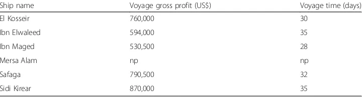
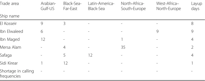
It goes without saying that any improvement in voyage gross profit or time in any trade area will affect the model optimal solution. This improvement may be caused by improvements in port dues and waiting time, cargo handling rate and charges, sailing time and fuel cost, and canal dues and transit time. Improvement may also be achieved by fair freight rates set by the marketplace for each trade area. For this research, im-provement is limited to Arabian-Gulf-US trade area only, caused by an imim-provement in port dues. This includes reduced dues for all tonnages and extra reduced dues for smaller ones. Refer to SOS (2018) for using SOS Voyager to enforce improvements other than port dues and time. Several improvements in port dues were tried through SOS Voyager and then passed to SOS Allocator to see the optimal improvement in voyage gross profit and time which may cause a shortage in calling frequencies in Arabian-Gulf-US trade area to disappear and layup days of Ibn Elwaleed and Ibn Maged to diminish; while maintaining maximum total port revenue. This optimal im-provement in voyage gross profit and time in Arabian-Gulf-US trade area is displayed in Table 15. Its corresponding optimal fleet calling frequencies in the year 2018, after improvement, is shown in Table 16. Total gross profit for all ships is $ 48,868,100.
The purpose of the analysis mentioned so far is to draw the attention to the chances to be taken in port development from the interest of both the ship owner and port op-erator simultaneously. The analysis is just proposing a shipping trade area improvement against an optimal calling frequency to be completed in this area. The analysis may eas-ily extend to ship types other than oil tankers. It also may extend to utilities other than ports; namely canals and straits. In case ESC fails to represent the oil shipping business, then SRC may either consider dummy tankers in an attempt to simulate real oil
Table 13Average voyage timea(days) in 2018, classified by ship and trade area
Trade area
Arabian-Gulf-USb Black-Sea-Far
–Eastb Latin-America-Black-Sea North-Africa-South-Europe West-Africa-North-Europe
Ship name
El Kosseir 30 24 17 npc 12
Ibn Elwaleed np np np 5 14
Ibn Maged np np np 5 11
Mersa Alam np 27 20 7 13
Safaga 32 26 18 np 15
Sidi Kirear 35 27 19 np 14
a
Average voyage time = Difference between calling date at first port and operation ending date at last port + voyage fixed time
b
In Arabian-Gulf-US trade area, ships do not pass Suez Canal; while in Black-Sea-Far-East trade area, ships pass Suez Canal
c
shipping business or, assemble results of ESC-like companies in an effort to reach a glo-bal solution for port development. In both cases, SOS-like systems remain the tool in doing this. In case the port is servicing more than one ship type, the conflict between types of services is not assumed in this research paper.
It takes SOS Allocator 1 second to process the model. Hardware used is Intel i3 PC. Software used are MS Windows 7, MS Access 2007 (front end), MS SQL Server 2008 (back end), and Microsoft Message Passing Interface (for parallel processing). No limits are imposed by SOS on number of ships or the number of trade areas.
Ship Appraiser
The following subsection describes the SOS Appraiser model, followed by a subsection to demonstrate a case study.
Ship Appraiser model
If one of the fleet units allocated by SOS Allocator is a new ship to be appraised for purchasing, building, or chartering-in, and such an allocation is tried for each year of the ship’s lifetime, SOS Appraiser may then be used in appraising its worthiness. SOS Appraiser aims at discounting ship gross profit plus other cash flow data obtained throughout ship lifetime and comparing the discounted value with the price of the ship. The model is displayed in Appendix 3. The model contains the Net Present Value for-mula, which unlike other NPV formulas can produce three net present values. This is attributed to the fact that cargo transport demand in tramp shipping is considered sto-chastic for many cargoes, if compared to liner shipping. For stosto-chastic cargo transport demand, SOS Voyager can calculate a voyage gross profit corresponding to demand
Table 14Optimal fleet calling frequencies in 2018, classified by ship and trade area
Trade area
Arabian-Gulf-US
Black-Sea-Far-East
Latin-America-Black-Sea
North-Africa-South-Europe
West-Africa– North-Europe
Layup days
Ship name
El Kosseir 10 2 - - - 2
Ibn Elwaleed - - - - 9 219
Ibn Maged - - - 36 - 165
Mersa Alam - 13 - - - 4
Safaga 9 1 2 - -
-Sidi Kirear - 7 9 - -
-Shortage in calling frequencies
9 1 1 - -
-Table 15Improved voyage gross profit and time in Arabian-Gulf-US trade area, classified by ship
Ship name Voyage gross profit (US$) Voyage time (days)
El Kosseir 760,000 30
Ibn Elwaleed 594,000 35
Ibn Maged 530,500 28
Mersa Alam np np
Safaga 790,500 32
upper limit (best case scenario), deterministic-equivalent value (most likely case), and lower limit (worst case). The three values of gross profit are passed to SOS Allocator and then to SOS Appraiser to calculate the three net present values.
As it is now clear, SOS Voyager followed by SOS Allocator is used to calculate the yearly gross profit needed by SOS Appraiser model. Programming algorithms used to solve SOS Voyager optimisation models permit the ship owner to change model parameters after optimisation without the need to re-optimise them from the beginning. This permits ship owner to easily change parameters such as cargo freight rate and quantity, port cargo handling rate and charges, and ship speed and fuel consumption, to see the effect of this change on the optimal solution. This permits the ship owner to validate the models used by SOS Voyager. In the sensi-tivity analysis, series of changes are given to SOS Voyager to see how far these changes are effective. In what-if analysis, a single change, in an interactive mode, is input to SOS Voyager to see the effect of this change on the objective function. Speed sensitivity or what-if analysis may be applied to all transport links, collect-ively, or to selective transport links, separately. Clicking menu options is all that is needed to perform optimisation, sensitivity, and what-if analysis. When a new ship is appraised, SOS Voyager is used to calculate its gross-profit-per-day for each voy-age completed on each trade area, along with sensitivity and what-if analysis of cargo quantity and freight. Since ship appraisal model cares for futuristic values of its parameters, stochastic rather than deterministic cargo transport demand is considered, especially in the case of tramp shipping. Three sensitivity and what-if analysis levels are identwhat-ified for the stochastic cargo transport demand: an upper limit, a deterministic-equivalent value, and a lower limit. To enable such analysis to take place, SOS Voyager archives data of every cargo offer for as long time as it takes to identify the behavior pattern of cargo quantity and freight. In the light of this pattern along with the forecast of future events that might affect it, a probability distribution of cargo transport demand may now be built and maintained.
The net present value formula is well-known and can be found everywhere in the in-vestment literature (take Evans and Marlow 1990 as one reference). However, the con-tribution made in the above-mentioned model is in the formulation of its objective function as it includes gross profit generated from integrated systems like SOS Voyager
Table 16Optimal fleet calling frequencies in 2018, after improvement, classified by ship and trade area
Trade area
Arabian-Gulf-US
Black-Sea-Far-East
Latin-America-Black-Sea
North-Africa-South-Europe
West-Africa– North-Europe
Layup days
Ship name
El Kosseir 9 3 - - - 8
Ibn Elwaleed 6 - - - 9 9
Ibn Maged 12 - - 1 - 4
Mersa Alam - 4 - 35 - 2
Safaga - 5 12 - - 4
Sidi Kirear 1 12 - - - 1
Shortage in calling frequencies
-and SOS Allocator. SOS Voyager creates input voyage parameters needed by SOS Allo-cator, and then SOS Allocator generates the yearly gross profit based on the trade area allocated to new ships in fair competition with already existing ones. The contribution is also made by the calculation of three net present values based on three levels of the stochastic cargo transport demand, as described in the following section.
Case study on ship Appraiser
The purpose of this case is to show the application of the model mentioned in the first subsection and sensitivity and what-if analysis referred to in this subsection. Assume that the shipping company ESC owns five oil tankers, working in tramp shipping busi-ness. To prepare the operational plan for the year 2019, ESC decided to re-allocate the five ships to oil trade areas, based on the gross profit each ship could earn in each area. A sixth oil tanker named El Kosseir was added to the plan as ESC is considering the purchase of this ship. For this purpose, ESC tried to figure out different voyages for each ship, one on each trade area. Stochastic cargo transport demand (quantity and freight rate) was then anticipated for a most-likely voyage most presenting each trade area. Demand is classified in three classes: upper limit, deterministic-equivalent value, and lower limit. SOS Voyager was then run to calculate voyage gross profit for each ship, including the new ship, on each trade area, using sensitivity and what-if analysis to calculate the gross profit for each demand class. Voyages failed to earn any gross profit were discarded. SOS Allocator was then run to see, for each demand class, what ship best fits in which trade area, and the frequency of calls it best completes in this trade area. This process results in a yearly gross profit for each ship for each demand class. Gross profit results for El Kosseir are reported in Table 17, along with similar re-sults for the years until 2028. Cash flow data other than gross profit is also reported in this table. El Kosseir investment data is reported in Table 18.
SOS passes data in Tables 17 and 18 to SOS Appraiser as to appraise the purchase of El Kosseir. It calculates, according to the model mentioned in the first subsection, the net present values corresponding to the cargo stochastic transport demand upper limit,
Table 17Yearly gross profit and cash flow data of El Kosseir in the period 2019-2028
Year Yearly gross profit in US$, based on stochastic cargo transport demand: Other yearly cash flow in US$
upper limit deterministic-equivalence lower limit
2019 7,245,200 6,825,300 6,221,200 1500,000
2020 7,832,100 7,120,000 6,514,100 1,750,000
2021 8,464,000 7,870,000 7,143,000 1,900,000
2022 9,182,000 8,560,000 7,932,000 2,100,000
2023 10,291,000 9,330,000 8,722,000 2,400,000
2024 11,024000 10,200,000 9,670,000 2,700,000
2025 11,694,000 10,970,000 10,472,000 3,050,000
2026 12,598,000 11,880,000 11,507,000 3,450,000
2027 13,610,000 12,740,000 12,530,000 3,850,000
deterministic-equivalence, and lower limit as follows: $ 17,483,560, $ 13,634,102, and $10,558,826, respectively. This result tells the ship owner that net present value is going to lie between the indicated lower and upper limits, and most likely it will be close to the indicated deterministic-equivalent value.
It takes SOS Appraiser a fraction of a second to process the model. Hardware used is Intel i3 PCs. Software used are MS Windows 7, MS Access 2007 (front end), MS SQL Server 2008 (back end), optimisation programs, and Microsoft Message Passing Inter-face (for parallel processing).
Concluding statement
This concluding statement is to bring about the contribution made in this paper; which is to announce a new policy to all systems which are sensitive to time. In tramp cargo transportation, as an example, the current policy is to select for each transport unit the cargo mix which contributes more to a gross-profit objective, assuming deterministic cargo transport demand. Since tramp cargo transportation system is sensitive to time, where time varies considerably from one alternative ship voyage to another, a new policy would consider this objective as less profit-able than gross-profit-per-day objective, assuming both deterministic and stochas-tic cargo transport demand. Owners of tramp transportation systems should worry not only about gross profit they expect to earn but also about the time taken in earning this profit. To introduce this new policy, SOS; a suite of deci-sion support systems, is developed to optimise tramp shipping operations using a stochastic gross-profit-per-day objective. This new objective has been introduced in SOS Voyager section by a model developed for ‘optimisation of ship voyage’ research area. The analysis given by this section demonstrates the case where the deterministic gross-profit objective is considerably less profitable for tramp ship-ping than that given by the stochastic gross-profit-per-day objective. Therefore, the following new management policy is set for any time-sensitive cargo transpor-tation system:
a) Use gross profit per day objective, rather than gross profit only.
b) Consider deterministic and stochastic cargo transport demand, rather than deterministic demand only.
c) Apply optimisation methods and use sensitivity and what-if analysis to validate the optimal solution.
In other words, old management policy of using gross-profit objective is not ad-vised any more, even if stochastic transport demand is absent. In case the
Table 18El Kosseir investment data
Investment data item Value in US$
Cost of investment in US$ 24,700,000
Risk-based rate of return in % 7
probability distribution cannot be identified for cargo transport demand, sensitivity and what-if analysis of cargo quantity and freight can be used with the gross-profit-per-day objective.
The impact of the new policy on any logistics and supply chain system is that it maintains the shortest possible transportation time the transportation system can afford. Findings of this part of the research paper can easily be extended to transportation systems other than cargo ships; namely cargo airplanes, trucks, and trains.
In SOS allocation model, it was shown that the optimal gross profit generated for each ship in each trade area can be used by SOS to allocate ships’ voyages to world cargo trade areas within a long-term planning period. One useful application of this al-location is to consider the frequency of calls allocated in each trade area as representing demand of services provided in this area and use this demand to assess the competi-tiveness of utilities in cargo trade areas. Ports are taken as an example for such utilities. The analysis given by the case study on port development demonstrates the case where an optimal trade area improvement is advised by SOS Voyager and SOS Allocator so that all calling frequencies in this area are serviced and ship layups are avoided, while maintaining maximum revenue of area ports. Sensitivity and what-if analysis is the SOS tool to reach this optimal trade area improvement. Findings of this part of the research paper can easily be extended to other ship types, other port services, other utilities; namely canals and straits.
Another useful application of SOS Allocator is that it calculates the gross profit of the new ship each year of its lifetime when it is added to old fleet units in the allocation plan. SOS Appraiser, as described in SOS Appraiser section, can then calculate three appraisal values, corresponding to three levels of stochastic cargo transport demand: an upper limit, deterministic-equivalence, and lower limit. The case study in this section calculates the three net present values for an oil tanker to be purchased for tramp shipping service and demonstrates how the deterministic-equivalent value represents the most likely value in a range of values bounded by lower and upper limits.
The contribution of this paper is not only in developing a decision support system using innovative models and methodologies for tramp shipping optimisation, but also in the integration it provides between these models and methodologies. The integration between SOS Voyager and SOS Allocator permits an exchange of parameters like voy-age gross profit to SOS Allocator and advisable working trade areas to SOS Voyvoy-ager. A next year planning budget is an important product which could be produced from this integration. Likewise, integration between SOS Allocator and SOS Appraiser permits calculation of gross profit of new ships and passing it to SOS Appraiser. SOS may be tried and manipulated by free download from SOS (2018). The site contains all SOS data, programs, and user manuals. SOS similar systems may be tailored for other means of cargo transport.
models need more attention. Cargo transport demand needs more study on the con-struction of probability distribution of the transport demand for main types of cargo. OR-Based Decision Support Systems are used to integrate OR models into database management systems. It is highly recommended to build such systems for shipping so that OR methodologies become transparent to ship owners while being supportive at the same time. Moreover, these systems have to interact with the ship owner in friend-lier sensitivity and what-if analysis sessions. Because hardware speed represents the prime limitation of the algorithm adopted in this paper, faster computer hardware and communication equipment must be used to enable ship owners take their decisions in the right time. Ship owners, operators of utilities, and researchers are encouraged to meet somewhere to discuss problems of mutual concern. It is highly recommended that workshops are to be considered as the places where all should meet to discuss case studies like the ones mentioned in this research paper. It is the role of international conferences to arrange such workshops in different places worldwide. The future work on tramp shipping should result in an impact on the logistic system in which transportation by ship is part of. An example of this impact is given by this re-search paper when it shows that shortening ship voyage time, to the extent ship owners can afford, is caused by a stochastic gross-profit-per-day objective. Finally, stochastic gross-profit-per-day objective may be used in other time-sensitive pro-duction systems. Examples are crop charts in agriculture, customized propro-duction line in industry, product maintenance schedule in services, project plan in con-struction, and logistics network in trade. It may be used as well in fixed-time pro-duction systems, before time being fixed, to determine the optimal amounts of factors of production employed in a multiple-products multiple-systems investment plan. Examples are crop harvesting in agriculture, car manufacturing and assembly lines in industry, port cargo handling in services, road paving in construction, and market control measurements in trade.
Appendix 1
SOS Voyager optimisation model
In this model, it is assumed that each ship starts its voyage at home port (open event) and returns back to its home port (close event). In this model let:
S= {1, 2, 3,…,s0} be the set of ships,
P= {1, 2, 3,…,p0} be the set of ports of a working trade area,
Q= {1, 2, 3, …,q0} be the set of cargoes available for transport between ports of this area. It is assumed that cargoes are compatible with the ship carrying them and can be mixed together on board the ship with ship stability maintained. Each cargor∈Qhas a loading event and a discharging event,
L= {1, 2, 3, …,l0} be a set of loading events, one for each cargo,
D= {1, 2, 3, …,d0} be a set of discharging events, one for each cargo,
F= {f} be a one-element set of open eventf,
G= {g} be a one-element set of close eventg,
E=L∪Dbe the set of load and discharge events, combined,
Ef=E∪Fbe the set of open, load, and discharge events, combined,
Efg=Ef∪Gbe the set of open, load, discharge, and close events, combined.
pibe portp∈Pidentified at eventi∈Efg,
Z= {1, 2, 3, 4} be an index representing two combined positions:‘pass or bypass Suez or Panama Canal’ as alternative route position, and ‘laden or ballast’ as ship load position. Z element of ‘1’ represents ship passing canal while in laden position,‘2’ represents ship bypassing canal while in laden position, ‘3’ represents ship passing canal while in ballast position, and ‘4’ represents ship bypassing canal while in bal-last position.
pk
ijz be the gross profit earned by shipk∈Son transport linkijwhile in positionz∈Z. Gross profit equals freight plus demurrage (based on reversible or irreversible calcula-tion), minus cooling/heating cost of cargo r∈Qat i∈L, minus handling cost of cargo
r∈Q at i∈E, minus dispatch (based on reversible or irreversible calculation), minus port dues of portp∈Pati∈Ef, wherepi≠pj, and minus canal/strait dues and fuel con-sumption of main engine when sailing transport link ij while in position z∈Z, where
pi≠pj,
Tk
g be voyage close day of shipk∈S,
Ckg be the cost of fuel consumption of auxiliary engine per day plus daily fixed cost of
shipk∈S,
Ck0 be voyage fixed cost of shipk∈S, not considered elsewhere,
xk
ijz be the problem decision variable. It equals 1 if ship k∈S sails transport link ij while it is in position z∈Z, and it equals zero otherwise. If xkijz = 1 andi∈E, cargor∈
Qis loaded on board shipk, whereiis its loading port, or discharged from the ship ifi
is its discharging port. Likewise, if xkijz = 1 and j∈E, cargo r∈Q is loaded on board
shipk, wherejis its loading port, or discharged from the ship ifjis its discharging port,
yibe another problem decision variable, alternative to xk
ijz. It may equal 1 ifxkijz = 0 for all ships sailing all transport links to pick up cargo r∈Qat i∈L, and it equals zero otherwise. Cargo r∈Q at i∈L is transported by a chartered-in ship in case it equals 1. For the chartered-in ship, let Pi be its voyage gross profit, ti be its voyage time, Ci0 be its voyage fixed cost, and ti0 be its voyage fixed time. Each one of these parameters is to have a value ≠0 if the chartered-in ship is taken as an alter-native and a value = 0 otherwise,
It is required to maximise the sum of voyage gross profit per day for all ships, given by:
G¼X k∈S
X i∈Ef
X j∈Eg
X z∈Zp
k
ijzxkijz−Cgk Tkg−Ck0
= Tk gþ
X
i∈LðPiyi−Ci0Þ=ðtiyiþti0Þ ð1Þ
Subject to:
Flow constraints
Using the above-mentioned denotations, the flow constraints can be formulated as follows: