R E S E A R C H
Open Access
A high-accuracy compact conservative
scheme for generalized regularized
long-wave equation
Xintian Pan
1,2*, Haitao Che
2and Yiju Wang
1*Correspondence:
1School of Management, Qufu
Normal University, Rizhao Shandong, 276800, China
2School of Mathematics and
Information Science, Weifang University, Weifang, 261061, China
Abstract
In this article, we develop a high-order compact conservative numerical scheme to solve the initial-boundary problem of GRLW equation. The proposed scheme is three-level and linear-implicit based on a finite difference method. A detailed numerical analysis of the scheme is presented including a convergence analysis result. Some numerical examples are provided to show the present scheme is efficient, reliable, and of high accuracy.
Keywords: GRLW equation; compact conservative scheme; solvability; convergence; stability
1 Introduction
The Cauchy problem of the generalized regularized long-wave (GRLW) equation reads
ut–βuxxt+ux+α
upx= , (.)
u(x, ) =u(x), (.)
whereα,βare positive constants andpis a positive integer []. The GRLW equation was first put forward by Peregrine [] and Benjaminet al.[] as a model for small-amplitude long waves on the surface of water in a channel. Many authors [–] have recently stud-ied models for long waves in nonlinear dispersive systems. Whenp= , (.) is usually called the RLW equation. Whenp= , (.) is called a modified regularized long-wave (MRLW) equation. Various numerical techniques have been developed to solve the equa-tion. These partly include the finite difference method, finite element methods, the least squares method, and a collocation method with quadratic B-splines, cubic B-splines and septic splines; we refer to [–], and references therein.
In general, the solutions of the system (.)-(.) decays rapidly to zero for |x| . Therefore, numerically we can solve the system (.)-(.) in a compact domain= (xl,xr) with –xl andxr. We can add the boundary conditions to the Cauchy problem (.)-(.),
u(xl,t) =u(xr,t) = . (.)
It is well known that the system (.)-(.) possesses the following conservative law:
E(t) =uL+uxL=E(). (.)
In [], Zhang considered a linear conservative scheme for GRLW equation, however, the accuracy of the scheme is only second-order. Recently, there has been growing in-terest in high-order compact methods to solve the partial differential equations [– ], where fourth-order compact finite difference approximation solutions for the tran-sient wave equations, a N-carrier system, the Klein-Gordon equation, the Sine-Gordon equation, the one-dimensional heat and advection-diffusion equations, the Schrödinger equation, the Klein-Gordon-Schrödinger equation and the RLW equation were shown, respectively. These numerical methods may give us many enlightenments to design a new numerical scheme for the GRLW equation. For a wide and most complete vision concern-ing the importance, the breadth, and the interest of the topics covered, we should also recall the study done on the long waves in [–].
The main purpose of this paper is to construct a new numerical scheme which has the following advantages:
. Coupling with the Richardson extrapolation, the new scheme is high-accuracy and without refined mesh; it has an accuracy ofO(τ+h).
. The new scheme is linearized and preserves the original conservative property. . The coefficient matrices of the scheme is symmetric and pentadiagonal, and the
Thomas algorithm can be employed to solve it effectively.
. Useful numerical examples are given to show the efficiency of the scheme.
The rest of this paper is organized as follows. In Section , a high-accuracy linear-compact difference scheme for the GRLW equation is described. In Section , we discuss the solvability of the scheme and the estimate of the difference solution. In Section , the fourth-order convergence and stability of the scheme are proved by the discrete energy method. Numerical results are reported in Section .
2 High-accuracy compact scheme and its discrete conservative law
In this section, we describe a high-order linear-compact difference scheme for (.)-(.). Let h=xr–xl
J andτ = T
N be the uniform step size in the spatial and the temporal di-rection, respectively. Denote xj=jh(≤j≤J),tn=nτ (≤n≤N),unj ≈u(xj,tn) and Z
h={u= (uj)|u–=u=uJ=uJ+= ,j= , , . . . ,J}. For simplicity, we introduce the fol-lowing notations of the difference operators:
δxunj = un
j+–unj
h , δx¯u n j =
un j –unj–
h , δxˆu n j =
un j+–unj–
h , δx¨u n j =
un j+–unj–
h ,
δˆtunj =u n+ j –unj–
τ , δtu n j =
un+ j –unj
τ , u¯ n j =
un+ j +unj–
.
Based on the notations above, we consider the following high-accuracy linear-compact scheme for the initial-boundary problem (.)-(.),
δˆtunj –
βδxδx¯δtˆu n j +
βδxˆδxˆδtˆu n j +
δˆx
unj– δ¨x
unj
+ p p+ α
δxˆu¯nj
unjp–+δˆx
unjp–u¯nj
–
δ¨xu¯nj
unjp–+δ¨x
unjp–u¯nj = ,
≤j≤J– , ≤n≤N– , (.)
uj– βδxδx¯u
j+
βδxˆδxˆu
j
=u(xj) – du
dx (xj) –τ
du
dx(xj) –τ αpu p– (xj)
du
dx (xj), (.)
uj =u(xj), ≤j≤J, (.)
un=unJ = , ≤n≤N. (.)
For convenience, the last term of (.) is defined by
κun,u¯n=κ
un,u¯n+κ
un,u¯n, (.)
where
κ
un,u¯n= p (p+ )α
δˆxu¯n
unp–+δxˆ
unp–u¯n, κ
un,u¯n= – p (p+ )α
δx¨u¯n
unp–+δx¨
unp–u¯n.
Theorem . Suppose u∈H[xl,xr],then the scheme(.)admits the following invariant:
En= u
n+
+un+ βδxu
n+
+δxun
– βδxˆu
n+
+δxˆun
+ hτ
J–
j=
δxunjunj+– hτ
J–
j=
δx¨unjunj+=En–=· · ·=E. (.)
Proof Taking in (.) the inner product with u¯nand using the boundary condition (.) yield
τu
n+–un–+ τβδxu
n+–δ xunx–
– τβδxˆu
n+–δ
ˆ
xunx–
+
δxun, u¯n
–
δx¨un, u¯n
Notice that
δxun, u¯n
= h J– j=
δxunjunj+–unjδxunj–
(.) and
δ¨xun, u¯n
= h J– j=
δ¨xunjunj+–unjδx¨unj–
. (.)
Now, computing the last term of the left-hand side in (.), we have
κ
un,u¯n, u¯n= p (p+ )αh
J–
j=
unjp–δˆx
¯
unj+δxˆ
unjp–u¯nju¯nj
= p (p+ )α
J–
j=
unjp–u¯nj+u¯nj –unj+p–u¯nj+u¯nj
– p (p+ )α
J–
j=
unj–p–u¯nju¯nj––unjp–u¯nju¯nj–
= . (.)
Similarly to the proof of (.), we get
κ
un,u¯n, u¯n= . (.)
Substituting (.)-(.) into (.). Let
En= u
n++un+ βδxu
n++δ xun
–
βδxˆu
n++δ
ˆ
xun
+ hτ
J–
j=
δxunjunj+– hτ
J–
j=
δx¨unjunj+.
By the definition ofEn, (.) follows.
3 Solvability and estimate for the difference solution
In this section, we shall discuss the estimate for the difference solution and the solvability of the difference scheme (.). For∀vn,wn∈Z
h, we define the discrete inner products and norms onZ
h via
vn,wn=h J–
j=
vnjwnj, δxvn,δxwn
l=h J–
j=
δxvnjδxwnj, vn
=vn,vn,
δxvn=
δxvn,δxvn
l, δx¨v
n=δ
¨
xvn,δx¨vn
l, v n
∞=≤maxj≤J–vnj.
Lemma .([]) For a mesh function u∈Zh,by the Cauchy-Schwarz inequality,we have
δx¨u≤ δxˆu≤ δxu.
Lemma .(Discrete Sobolev’s inequality []) There exist two constants Cand Csuch that
un∞≤Cun+Cδxun.
Theorem . Suppose that u∈H,then there is the estimation for the solution unof the scheme(.):un ≤C,δxun ≤C,which yieldsun∞≤C.
Proof It follows from (.) and the Cauchy-Schwartz inequality that
u
n++un+ βδxu
n++δ xun
–
βδxˆu
n++δ
ˆ
xun
≤C+ hτ
J–
j=
δxunjunj++ hτ
J–
j=
δx¨unjunj+
≤C+ τδxu
n
+un++ τδx¨u
n
+un+. (.)
According to Lemma ., we obtain from (.)
– τ
un++un +
βδxun+
+
β– τ
δxun
≤C. (.)
This implies for smallτwhich satisfiesβ–τ> that we have
un≤C, δxun≤C. (.)
Using Lemma ., we obtain
un∞≤C. (.)
Remark . Theorem . implies that the scheme (.) is unconditionally stable.
Theorem . The difference scheme(.)is uniquely solvable.
Proof Let us prove the unique solvability by induction. It is obvious thatuandu are uniquely determined by (.) and (.), respectively. Suppose thatu,u, . . . ,unbe solved uniquely. Considerun+in (.) which satisfies
τu
n+ j –
τβδxδ¯xu
n+ j +
τδˆxδˆx
unj++ p (p+ )α
unjp–δxˆunj++δxˆ
unjp–unj+
– p
(p+ )
unjp–δx¨unj++δx¨
Taking the inner product of (.) withun+, we obtain
τu
n++ τβδxu
n+– τβδxˆu
n++I–II,un+= , (.)
where
I= p (p+ )α
unjp–δxˆunj++δxˆ
unjp–unj+,
II= p (p+ )
un j
p–
δx¨unj++δ¨x
un j
p– un+
j
.
Similarly to the proof of (.), we get
I,un+= , II,un+= . (.)
It follows from (.)-(.) and Lemma . that
τu
n++ τβδxu
n+≤. (.)
That is, (.) has only a trivial solution. Hence, (.) determinesunj+uniquely. This
com-pletes the proof of Theorem ..
4 Convergence and stability of the difference scheme
First, we shall consider the truncation error of the difference scheme (.)-(.). Letvn j = u(xj,tn). We define the truncation error as follows:
Erjn=δˆtvnj –
βδxδx¯δˆtv n j +
βδxˆδxˆδtˆv n j +
δxˆ
vnj– δx¨
vnj
+ p p+ α
δxˆv¯nj
vnjp–+δxˆ
vnjp–v¯nj
–
δx¨v¯nj
vnjp–+δx¨
vnjp–v¯nj ,
≤j≤J– , ≤n≤N– , (.)
sj =vj– βδxδx¯v
j+
βδxˆδxˆv
j–u(xj)
+d u
dx (xj) +τ
du
dx (xj) +τ αpu p– (xj)
du
dx(xj), (.)
vj =u(xj), ≤j≤J, (.)
vn
=vnJ = , ≤n≤N. (.)
Using a Taylor expansion, we obtain|Ern|+|s|=O(τ+h) holds ifτ,h→. Next, we shall discuss the convergence and stability of the scheme (.)-(.).
Lemma .(Discrete Gronwall inequality []) Suppose that the discrete mesh function
{wn|n= , , . . . ,N;Nτ=T}satisfies the recurrence formula
where A,B,and Cn(n= , . . . ,N)are nonnegative constants.Then
wn∞≤
w+τ N
k= Ck
e(A+B)T,
whereτ is small,such that(A+B)τ≤NN–(N> ).
Theorem . Assume that u∈H,then the solution unof the scheme(.)-(.)converges to the solution of the initial-boundary problem (.)-(.)and the rate of convergence is O(τ+h)by the ·
∞norm.
Proof Letenj =vnj –unj. From (.)-(.) and (.)-(.), we have
Erjn=δˆtenj –
βδxδ¯xδˆte n j +
βδˆxδˆxδˆte n j +
δxˆ
enj– δ¨x
enj
+ p p+ α
δxˆv¯nj
vnjp–+δxˆ
vnjp–v¯nj
–
δxˆu¯nj
unjp–+δxˆ
unjp–u¯nj
– p p+ α
δx¨v¯nj
vnjp–+δx¨
vnjp–¯vnj
–
δx¨u¯nj
unjp–+δx¨
unjp–u¯nj , ≤j≤J– , ≤n≤N– , (.)
sj =ej– βδxδ¯xe
j+
βδˆxδˆxe
j, (.)
ej = , ≤j≤J, (.)
en=enJ = , ≤n≤N. (.)
Taking in (.) the inner product with e¯n(i.e. en++en–), we obtain
Ern, ¯en=δˆten
+ βδˆtδxe
n –
βδˆtδxˆe n
+ h J– j=
δxenjenj+–enjδxenj–
– h J– j=
δx¨enjenj+–enjδx¨enj–
+P+P+Q+Q, ¯en
, (.)
where
P= pα (p+ )
δxˆv¯n
vnp––δxˆu¯n
unp–,
P= pα (p+ )
δxˆ
vnp–v¯n–δxˆ
unp–u¯n, Q= –
pα (p+ )
δ¨xv¯n
vnp––δx¨u¯n
unp–,
Q= – pα (p+ )
δx¨
vnp–v¯n–δx¨
Computing the sixth term on the right-hand side of (.) and using Lemma . and The-orem . yield
P, e¯n
= pα (p+ )
δxˆv¯n
vnp––δxˆu¯n
unp–, e¯n
= pα (p+ )
δxˆe¯n
vnp–+δxˆu¯n
vnp––unp–,¯en
= pα (p+ )h
J–
j=
δxˆe¯nj
vnjp–¯enj + J–
j=
δxˆu¯nj
vnjp––unjp–e¯nj
= pα (p+ )h
J–
j=
δxˆe¯nj
vnjp–¯enj + J–
j=
δˆxu¯nj
enj p–
k=
vnjp––kunjk
¯
enj
≤Cδxˆe¯n
+en+e¯n
≤Cδxen+
+δxen–
+en++en+en–, (.)
where the Cauchy-Schwartz inequality and Lemma . are used. Similarly, we can also obtain
P, e¯n≤Cδxen+
+δxen–
+en++en+en–, (.)
Q, e¯n
≤Cδxen+
+δxen–
+en+
+en+en–
, (.)
Q, ¯en
≤Cδxen+
+δxen–
+en++en+en–. (.)
In addition, it is obvious that
Ern, ¯en≤Ern+ e
n++en–, (.)
h J– j=
δxenjenj+–enjδxenj–
≤Cδxen
+δxen–
+en++en, (.)
– h J– j=
δx¨enjenj+–enjδx¨enj–
≤Cδxen
+δxen–
+en++en. (.)
It follows from (.)-(.) that
δˆten
+ βδˆtδxe
n– βδtˆδxˆe
n
≤Ern+Cδxen+
+δxen
+δxen–
+en++en+en–. (.)
LetBn=
(en++en) +
β
(δxen++δxen). Using Lemma ., (.) can be written as follows:
According to Lemma ., we can immediately obtain
Bn≤
B+T sup l≤n≤N
Ern
eCT. (.)
Taking the inner product of (.) witheyields
s,e=e+ βδxe
–
βδx¨e
. (.)
This, together with (s,e)≤(s+e),|s|=O(τ+h), and Lemma ., gives
e≤Oτ+h, δ
xe≤O
τ+h. (.)
From the discrete initial condition (.), we know thatB= [O(τ+h)]. It follows from (.) that
Bn≤Oτ+h. (.)
Then we have
en≤Oτ+h, δxen≤O
τ+h. (.)
This, together with Lemmas ., gives
en∞≤Oτ+h. (.)
This completes the proof of Theorem ..
Similarly, we can prove stability of the difference solution.
Theorem . Under the conditions of Theorem.,the solution of the scheme(.)-(.) is unconditionally stable by the · ∞norm.
5 Numerical experiments
In this section, we give some numerical experiments to demonstrate our theoretical results obtained in the previous sections. We will measure the accuracy of the proposed scheme using the absolute error defined byen=vn–un
∞.
Consider the initial-boundary value problem (.)-(.). In the numerical experiments, we takexl= –,xr= ,T= , and choose three casesp= , , , respectively. In order to verify the accuracyO(τ+h), we takeτandhsmall enough to verify the fourth-order accuracy and second-order accuracy in the spatial and temporal directions, respectively. The convergence order figures oflog(en)-log(h) withhand the ones oflog(en)-log(τ) with τ small enough are given in Figures - for various mesh stepshandτ att= . From Figures -, it is obvious that the scheme (.)-(.) is convergent in the maximum norm, and the convergence order isO(τ+h).
Figure 1 The spatial convergence order in maximal norm forunatt= 10 with differenthandτ computed by the scheme (2.1)-(2.4).
Figure 2 The temporal convergence order in maximal norm forunatt= 10 with differenthandτ
computed by the scheme (2.1)-(2.4).
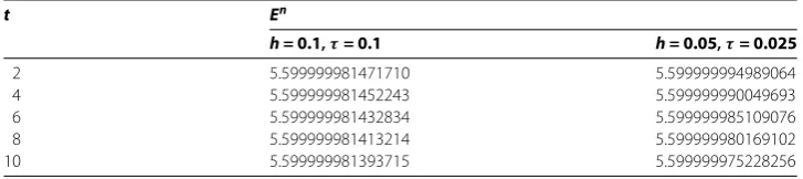
Table 1 Discrete energyEnof the scheme (2.1) at different timetwhenh= 0.1, 0.05 andp= 2
t En
h = 0.1,τ= 0.1 h = 0.05,τ= 0.025
2 5.599999981471710 5.599999994989064
4 5.599999981452243 5.599999990049693
6 5.599999981432834 5.599999985109076
8 5.599999981413214 5.599999980169102
10 5.599999981393715 5.599999975228256
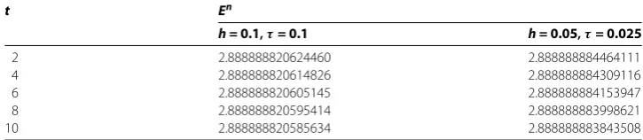
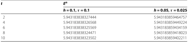
presented for three casesp= , , under various mesh stepshandτ, respectively. It is easy to see from Tables - that the scheme (.) preserves the discrete energy very well, which also shows the accuracy and efficiency of the scheme in this paper.
Case . Takep= . Consider the following initial-boundary problem of RLW equation:
ut–uxxt+ux+uux= , (.)
Figure 3 The spatial convergence order in maximal norm forunatt= 10 with differenthandτ computed by the scheme (2.1)-(2.4).
Figure 4 The temporal convergence order in maximal norm forunatt= 10 with differenthandτ
computed by the scheme (2.1)-(2.4).
Table 2 Discrete energyEnof the scheme (2.1) at different timestwhenh= 0.1, 0.05 andp= 3
t En
h = 0.1,τ= 0.1 h = 0.05,τ= 0.025
2 2.888888820624460 2.888888884464111
4 2.888888820614826 2.888888884309116
6 2.888888820605145 2.888888884153947
8 2.888888820595414 2.888888883998621
10 2.888888820585634 2.888888883843508
u(xl,t) =u(xr,t) = . (.)
Figure 5 The spatial convergence order in maximal norm forunatt= 10 with differenthandτ
computed by the scheme (2.1)-(2.4).
Figure 6 The temporal convergence order in maximal norm forunatt= 10 with differenthandτ computed by the scheme (2.1)-(2.4).
Table 3 Discrete energyEnof the scheme (2.1) at different timetwhen (h,τ) = (0.1, 0.1) and (0.05,0.025) forp= 4
t En
h = 0.1,τ= 0.1 h = 0.05,τ= 0.025
2 5.943183838327444 5.943183859464757
4 5.943183838326568 5.943183859449224
6 5.943183838325569 5.943183859434159
8 5.943183838324471 5.943183859418023
10 5.943183838323502 5.943183859402211
Case . Takep= . We consider the following initial-boundary problem of MRLW equa-tion:
ut–uxxt+ux+
ux= , (.)
u(x, ) =u(x), (.)
In experiments, we choose the initial conditionu(x, ) =
√
sech(
x) []. The conver-gence order figures and the values ofEnare shown in Figures - and Table , respec-tively.
Case . Takep= . We consider the initial-boundary problem (.)-(.) of GRLW equa-tion:
ut–uxxt+ux+uux= , (.)
u(x, ) =u(x), (.)
u(xl,t) =u(xr,t) = . (.)
In the following experiments, we choose the initial conditionu(x, ) =sech(
√
x) []. The convergence order figures and the values ofEnare shown in Figures - and Table , respectively.
Competing interests
The authors declare that they have no competing interests.
Authors’ contributions
The article was carried out in collaboration between all authors. The three authors have contributed to, read, and approved the manuscript.
Acknowledgements
This work is supported by the Natural Science Foundation of China (No. 11201343, 11401438), Natural Science Foundation of Shandong Province (ZR2012AM017, ZR2013FL032), a Project of Shandong Province Higher Educational Science and Technology Program (No. J14LI52, J15LI56), the Youth Research Foundation of WFU (No. 2013Z11) and the Project of Science and Technology Program of Weifang (Grant no. 201301006).
Received: 25 May 2015 Accepted: 27 July 2015
References
1. Zhang, L: A finite difference scheme for the generalized regularized long-wave equation. Appl. Math. Comput.168, 962-972 (2005)
2. Peregrine, DH: Calculations of the development of an undular bore. J. Fluid Mech.25, 321-330 (1966)
3. Benjamin, TB, Bona, JL, Mahony, JJ: Model equations for long waves in nonlinear dispersive systems. Philos. Trans. R. Soc. Lond. A272, 47-78 (1972)
4. Albert, J: Dispersion of low-energy waves for the generalized Benjamin-Bona-Mahony equation. J. Differ. Equ.63(1), 117-134 (1986)
5. Ruggieri, M, Speciale, MP: Similarity reduction and closed form solutions for a model derived from two-layer fluids. Adv. Differ. Equ.2013, 355 (2013)
6. Lmaco, J, Clark, HR, Medeiros, LA: Remarks on equations of Benjamin-Bona-Mahony type. J. Math. Anal. Appl.328(2), 1117-1140 (2007)
7. Ruggieri, M, Speciale, MP: New exact solutions for a coupled KdV-like model. J. Phys. Conf. Ser.482, 012036 (2014) 8. Gear, JA, Grimshaw, R: Weak and strong interactions between internal solitary waves. Stud. Appl. Math.70, 235-258
(1984)
9. Kutluay, S, Esen, A: A finite difference solution of the regularized long wave equation. Math. Probl. Eng.2006, 1-14 (2006)
10. Zhang, L, Chang, Q: A new finite difference method for regularized long-wave equation. Chinese J. Numer. Methods Comput. Appl.23, 58-66 (2001)
11. Avilez-Valente, P, Seabra-Santos, FJ: A Petrov-Galerkin finite element scheme for the regularized long wave equation. Comput. Mech.34, 256-270 (2004)
12. Esen, A, Kutluay, S: Application of a lumped Galerkin method to the regularized long wave equation. Appl. Math. Comput.174(2), 833-845 (2006)
13. Guo, L, Chen, H:H1-Galerkin mixed finite element method for the regularized long wave equation. Computing77,
205-221 (2006)
14. Gu, H, Chen, N: Least-squares mixed finite element methods for the RLW equations. Numer. Methods Partial Differ. Equ.24, 749-758 (2008)
15. Saka, B, Dag, I: A numerical solution of the RLW equation by Galerkin method using quartic B-splines. Commun. Numer. Methods Eng.24, 1339-1361 (2008)
17. Dag, I, Ozer, MN: Approximation of the RLW equation by the least square cubic B-spline finite element method. Appl. Math. Model.25, 221-231 (2001)
18. Dag, I, Saka, B, Irk, D: Application of cubic B-splines for numerical solution of the RLW equation. Appl. Math. Comput. 159, 373-389 (2004)
19. Soliman, AA, Raslan, KR: Collocation method using quadratic B-spline for the RLW equation. Int. J. Comput. Math.78, 399-412 (2001)
20. Soliman, AA, Hussien, MH: Collocation solution for RLW equation with septic spline. Appl. Math. Comput.161, 623-636 (2005)
21. Cohen, G: High-Order Numerical Methods for Transient Wave Equations. Springer, New York (2002)
22. Dai, W: An improved compact finite difference scheme for solving a N-carrier system with Neumann boundary conditions. Numer. Methods Partial Differ. Equ.27, 436-446 (2011)
23. Dai, W, Tzou, DY: A fourth-order compact finite difference scheme for solving a N-carrier system with Neumann boundary conditions. Numer. Methods Partial Differ. Equ.25, 274-289 (2010)
24. Dehghan, M, Mohebbi, A, Asgari, Z: Fourth-order compact solution of the nonlinear Klein-Gordon equation. Numer. Algorithms52, 523-540 (2009)
25. Mohebbia, A, Dehghan, M: High-order solution of one-dimensional Sine-Gordon equation using compact finite difference and DIRKN methods. Math. Comput. Model.51, 537-549 (2010)
26. Mohebbia, A, Dehghan, M: High-order compact solution of the one-dimensional heat and advection-diffusion equations. Appl. Math. Model.34, 3071-3084 (2010)
27. Dehghan, M, Taleei, A: A compact split-step finite difference method for solving the nonlinear Schrodinger equations with constant and variable coefficients. Comput. Phys. Commun.181, 43-51 (2010)
28. Xie, S, Li, G, Yi, S: Compact finite difference schemes with high accuracy for one-dimensional nonlinear Schrödinger equation. Comput. Methods Appl. Mech. Eng.198, 1052-1060 (2009)
29. Wang, T, Guo, B: Unconditional convergence of two conservative compact difference schemes for non-linear Schrödinger equation in one dimension. Sci. Sin., Math.41(3), 207-233 (2011) (in Chinese)
30. Pan, X, Zhang, L: High-order linear compact conservative method for the nonlinear Schrodinger equation coupled with the nonlinear Klein-Gordon equation. Nonlinear Anal.92, 108-118 (2013)
31. Zheng, K, Hu, J: High-order conservative Crank-Nicolson scheme for regularized long wave equation. Adv. Differ. Equ. 2013, 287 (2013)
32. Alias, A, Grimshaw, RHJ, Khusnutdinova, KR: On strongly interacting internal waves in a rotating ocean and coupled Ostrovsky equations. Chaos23(2), 023121 (2013)
33. Ruggieri, M, Speciale, MP: KdV-like equations for fluid dynamics. AIP Conf. Proc.1637, 918-924 (2014)
34. Alias, A, Grimshaw, RHJ, Khusnutdinova, KR: Coupled Ostrovsky equations for internal waves in a shear flow. Phys. Fluids26, 126603 (2014)
35. Ruggieri, M, Speciale, MP: Quasi self-adjoint coupled KdV-like equations. In: 11th International Conference of Numerical Analysis and Applied Mathematics, vol. 1558, pp. 1220-1223. AIP, New York (2013)
36. Ruggieri, M, Speciale, MP: On a hierarchy of traveling wave solutions in a shallow stratified fluid. In: 11th International Conference of Numerical Analysis and Applied Mathematics, vol. 1558, pp. 1793-1796. AIP, New York (2013) 37. Zhou, Y: Application of Discrete Functional Analysis to the Finite Difference Method. Inter. Acad. Publishers, Beijing