R E S E A R C H
Open Access
Exponential and polynomial stabilization of
the Kirchhoff string by nonlinear boundary
control
Yuhu Wu
1*and Jianmin Wang
2*Correspondence:
1Department of Mathematics,
Harbin University of Science and Technology, Harbin, 150080, P.R. China
Full list of author information is available at the end of the article
Abstract
This paper addresses the stabilization problem of the nonlinear Kirchhoff string using nonlinear boundary control. Nonlinear boundary control is the negative feedback of the transverse velocity of the string at one end, which satisfies a polynomial-type constraint. Employing the multiplier method, we establish explicit exponential and polynomial stability for the Kirchhoff string. The theoretical results are assured by numerical results of the asymptotic behavior for the system.
1 Introduction
Stabilization and vibration controllability of string or beam systems arising from different engineering backgrounds has attracted attention of many researchers [–]. In particular, boundary feedback stabilization of string and beam systems has become an important re-search area [–]. This is because, in a practice system, vibration is more easily controlled through a boundary point than using point sensors or actuators away from the boundaries [, ].
There are several nonlinear mathematical models that describe the transversal vibration of stretched strings. One such model is presented in the following equation:
ytt(x,t) =
a+b
yx(x,t)dx
yxx(x,t) ()
for allx∈(, ) andt≥, wherea> ,b≥ are two constants. Obviously, the above equation is a simple prototype of the classical equation
ρhytt(x,t) =
T+ hE
l
l
yx(x,t)dx
yxx(x,t),
which was proposed by Kirchhoff []. Herelis the length of the string;Eis Young’s mod-ulus of the material;ρis density;his the area of the cross section;y(x,t) is the transversal displacement of the pointxof the string at timet. This model has been studied by re-searchers from the physical and mathematical points of view; see,e.g., references [–] and the references therein.
Figure 1 Schematic of the nonlinear Kirchhoff string with boundary control.
In this paper, we consider Kirchhoff string () with the following boundary conditions (see Figure ):
y(,t) = , ()
T(t)yx(,t) =u(t) ()
for allt≥.T(t) denotes the tension in the string at timet. The boundary condition in equation () implies that the string is fixed atx= . The boundary condition in equation () represents the balance of the transversal component of the tension in the string and the control inputuwhich is applied transversally atx= . Because the tension in the string represented by equation () is not constant and is given by
T(t) =a+b
yx(x,t)dx ()
for allt≥ (see []), the boundary condition in equation () can be written as
a+b
yx(x,t)dx
yx(,t) =u(t). ()
Shahruz and Krishna [] investigated the stabilization of Kirchhoff string () with a linear negative velocity control, which means the boundary controluhas a linear negative velocity feedback form
u(t) :=uyt(,t)
= –Lyt(,t) ()
for allt≥, whereLis a positive constant. They established exponential stability. In [], the absolute stability of the Kirchhoff string () with linear sector boundary control was considered. It is well known that linear strings represented by equation (), for whichb= , can be stabilized by the control law in equation (); seee.g., references [–]. Moreover, Shahruz [], Funget al.[], and Li and Hou [] developed linear boundary control laws for axially moving strings. It is worth mentioning that Kobayashi [] designed a linear parallel compensator based on boundary displacement observer and proved the string () can be stabilized by parallel compensator control.
direct method. In this work, we investigate the stabilization of string () with a more gen-eral and ‘flexible’ boundary control (see hypothesis (H) in Section ). The feedback func-tionuis not required to satisfy a strict control law such as (), but just satisfies some ap-propriate polynomial-type constraint. In this general boundary control case, it seems that the Lyapunov direct method is no more applicable. So, we need to use a more meticulous method to deal with the stabilization problem. Applying the multiplier method, we estab-lish not only exponential stability result but also polynomial stability result for Kirchhoff string ().
The remainder of this technical paper is arranged as follows. Section describes the model of the Kirchhoff nonlinear string and introduces the control assumption. The prob-lem of exponential and polynomial stability is addressed in Section . Finally, a numerical example is demonstrated where the nonlinear distributed parameter infinite-dimensional equation is solved by applying the finite element method in Section .
2 Problem formulation
Consider the nonlinear Kirchhoff string model as shown in Figure . For the sake of easy reading and later referring, the governing equation, the boundary conditions and the ini-tial functions are put together as
⎧ ⎪ ⎪ ⎪ ⎨ ⎪ ⎪ ⎪ ⎩
ytt(x,t) = [a+b
yx(x,t)dx]yxx(x,t), (a)
y(,t) = , (b)
[a+byx(x,t)dx]yx(,t) =u(yt(,t)), (c)
y(x, ) =f(x), yt(x, ) =g(x) (d)
for allx∈(, ) andt≥. Heref(x) andg(x) in equation (d) are the initial displacement and velocity of the string, respectively. We assume thatf∈C[, ],g∈C[, ] and that at
least one of the functionsf orgis not identically zero over [, ].
To obtain a precise stabilization result, we make the following hypothesis on the con-tinuous control feedbacku:R→R:
(H) There exist constantsL≥L> andr≥such that
u(w)∈(w) :=
–Co{Lw,Lw}, |w|> ,
–Co{Lwr,Lw
r}, |w| ≤. ()
Remark . Obviously, condition (H) is equivalent to, for allw∈R,
u(w)w≤,
Lmin{|w|,|w|r} ≤ |u(w)| ≤Lmax{|w|,|w|
r}.
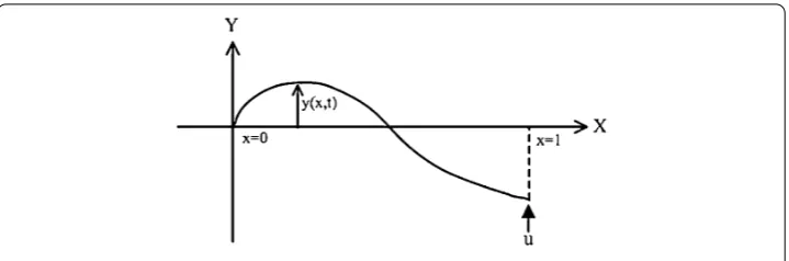
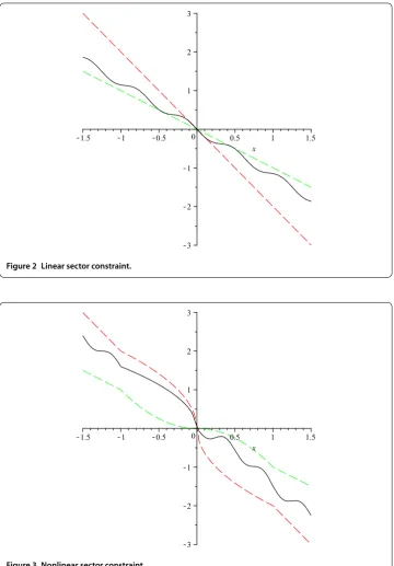
Obviously, hypothesis (H) is a ‘flexible’ and ‘robust’ condition, which allows the feed-back functionuto vary in an appropriate geometric region given by a polynomial-type constraint. For example, Figure illustrates a feedback controlusatisfying a linear sector constraint (H) withr= ,L= ,L= , and Figure shows a feedback controlusatisfying
a nonlinear constraint (H) withr= ,L= ,L= . Sinceu(yt(,t))yt(,t)≤, for allt≥, the boundary control (c) is the negative feedback of transversal velocity of the string at
Figure 2 Linear sector constraint.
Figure 3 Nonlinear sector constraint.
For the existence and uniqueness of the solution of the general Kirchhoff equation, we refer to [, ] and references therein. In this work, we study the stabilization of the string in (a) by this negative feedback boundary controlu, which provides a dissipative effect.
Remark . According to boundary condition (b) atx= , we easily get
We define the natural energy function of time for system (a)-(d) and denote it byt→ E(t). The scalar-valued functionEis defined as
E(t) :=
yt(x,t)dx+
ayx(x,t)dx+b
yx(x,t)dx
. ()
Especially, from the initial displacement and velocity condition (d), we obtain the initial energy as
E() =
g(x) +afx(x)dx+b
fx(x)dx
.
Since at least one of the functionsfandgis not identically zero over (, ) we haveE() > .
3 Stabilization by boundary control
In this section we state and prove our main result. For this purpose we establish several lemmas.
Lemma . Let y(·,·)be the solution for system(a)-(d).Then
yxyxtdx=yx(,t)yt(,t) –
yxxytdx, ()
xyxyxxdx= y
x(,t) –
yx(x,t)dx, ()
xyxyttdx=
[xyxyt]t+ y
t
dx– y
t(,t). ()
Proof See the Appendix.
Now, we give a property of the energy functionE.
Proposition . The time-derivative of the energy function E in equation(),along the solution of system(a)-(d)satisfies
E(t) =u(t)yt(,t)≤ ()
for all t≥.
Proof Differentiating the energy function () with respect tot, we get
E(t) =
ytyttdx+
a+b
yxdx
yxyxtdx. ()
According to equation () and boundary control (c), we get
a+b
yxdx
yxyxtdx
=u(t)yt(,t) –
a+b
yxdx
Substituting equation () into equation () and observing (a), we obtain
E(t) =u(t)yt(,t) +
yttytdx–
a+b
yxdx
yxxytdx
=u(t)yt(,t) ()
for allt≥. We obtain equation ().
Remark . From Proposition ., we obtain the energy identity for system (a)-(d),
E(S) –E(T) =
S T
u(t)yt(,t)dt.
Therefore, the energyEis a decreasing function of time.
During the subsequent stability analysis, we utilize the following inequality.
Lemma . Let y(·,·)be the solution for system(a)-(d).Then
xyx(x,t)yt(x,t)dx≤max
,
a
E(t) ()
for all t≥.
Proof Applying the Cauchy-Schwarz inequality, we get
xyx(x,t)yt(x,t)dx≤
xyxdx+
ytdx
≤
yxdx+
ytdx ()
for allt≥. On the other hand, the definition of energy function () implies
a
yxdx+
ytdx≤E(t)
for allt≥. It follows from the above inequality that
yxdx+
ytdx≤
E(t), a≥,
aE(t), <a< .
()
Together with () and (), we get equation (). Hence we complete the proof of
Lem-ma ..
Now, we present a Gronwall-type lemma (see Komornik [], pp.), which will play an essential role when establishing the stabilization result.
Lemma . Let G:R+→R+be a non-increasing function.Assume that there exists a con-stantω> such that
+∞
T
Gq+(t)dt≤
Then the following estimation is true,for all t≥,
G(t)≤G()e–ωt if q= ,
G(t)≤G()(+qωqt)q if q> .
We givea prioriestimation for the energy functionE(t), which was established in []. For the sake of completeness, we give the proof here.
Lemma . The energy function E in equation(),along the solution of system(a)-(d),
satisfies
E(t)≤–
[xyxyt]tdx+ y
t(,t) + au
y
t(,t)
()
for all t≥.
Proof We multiply equation (a) byxyx(x,t) and do integration over [, ], with respect tox. We obtain
=
xyx
ytt–
a+b
yxdx
yxx dx =
[xyxyt]t+ y
t
dx– y
t(,t)
–
a+b
yxdx
yx(,t) –
yxdx
, ()
using equations () and () in Lemma .. It follows from () that
ytdx+
a+b
yxdx
yxdx
=E(t) + b
yxdx
. ()
Sincea+by
xdx≥a, according to boundary control (c), we have
a+b
yxdx
yx(,t)≤
au y
t(,t)
. ()
Hence, substituting equation () into equation () and using equation (), one has
E(t) +b
yxdx
= –
[xyxyt]tdx+ y
t(,t) +
a+b
yxdx
yx(,t)
≤–
[xyxyt]tdx+ y
t(,t) + au
y
t(,t)
.
Lemma . For any constant q≥,the energy function E along the solution of system
(a)-(d)satisfies the following estimation,for all S>T≥,
S T
Eq+(t)dt≤CEq+(T) +
S T
Eq(t)yt(,t)dt
+ a
S T
Eq(t)uyt(,t)
dt, ()
where C=qq++max{,a}.
Proof According to inequality () in Lemma ., we have, for all ≤T<S,
S T
Eq+(t)dt≤–
S T
Eq(t)
[xyxyt]tdx dt
+
S T
Eq(t)yt(,t)dt+ a
S T
Eq(t)uyt(,t)
dt. ()
Moreover, using integration by parts, we get
S T
Eq(t)
[xyxyt]tdx dt=
S T
Eq(t)
xyxytdx
t dt – S T
qE(t)Eq–(t)
(xyxyt)dx dt.
Hence, inequality () becomes
S T
Eq+(t)dt≤A+A+
S T
Eq(t)yt(,t)dt
+ a
S T
Eq(t)uyt(,t)
dt, ()
where
A:= –
S T
Eq(t)
xyxytdx
t
dt,
A:=
S T
qE(t)Eq–(t)
(xyxyt)dx dt.
Firstly, we estimateAandA,
A = –
S T
Eq(t)
xyxytdx
t
dt
≤Eq(T)
xyx(x,T)yt(x,T)dx
+Eq(S)
xyx(x,S)yt(x,S)dx
(by ()) ≤max , a
Eq+(T) +max
,
a
Eq+(S)
≤max
,
a
where the last inequality follows from the factE(t) is a decreasing function. On the other hand,
A =
S T
qE(t)Eq–(t)
xyxytdx dt
≤
S T
qE(t)Eq–(t)
xyxytdx
dt
≤max
,
a
S
T
qE(t)Eq(t)dt (by ())
= q
q+ max
,
a
Eq+(S) –Eq+(T)
≤ q
q+ max
,
a
Eq+(T). ()
Finally, inserting the two inequalities, () and (), in (), we get inequality (). This
completes the proof of Lemma ..
We now state the main stabilization result for system (a)-(d).
Theorem . Assume that assumption (H) holds. Then there exist three constants k,k,σ> such that,for all t≥,
E(t)≤ke–σt if r= , E(t)≤kt–
r– if r> . ()
Remark . It is worth to mention that Theorem . in [] can be viewed as a special cases of Theorem .. Indeed, in the linear control case (), the exponential stability in Theorem . coincides with the result in [].
Proof of Theorem. We distinguish two cases related to the parameterrto establish the energy decay rate.
Case (I): r= ; Case (II): r> .
In Case (I), we chooseq= . According to hypothesis (H), we know that
s≤–
L
u(s)s, u(s)≤–Lu(s)s for alls∈R.
Hence, from inequality () and equation (), we deduce that, for allS>T≥,
S T
E(t)dt≤CE(T) +
S T
yt(,t) +
au y
t(,t)
dt
≤CE(T) –
a+LL
aL
S T
u(t)yt(,t)dt
=CE(T) +
a+LL
aL
S T
–E(t)dt
≤CE(T), ()
Now we deal with Case (II). In this case, we chooseq=r– > . We first admit the fol-lowing fact (the proof is given in the Appendix).
Claim For anyδ> ,we have the following estimates,for all S>T≥,
S T
Eq(t)y
t(,t)dt≤
r–
r+ δ r+ r–
S T
Eqrr+–(t)dt
+ δ
–r+
(r+ )L
E(T) + (q+ )L
Eq+(T), ()
S T
Eq(t)uy
t(,t)
dt≤r– r+ δ
r+ r–
S T
Eqrr–+(t)dt
+L r
δ–
r+ (r+ ) E(T) +
L
(q+ )E
q+(T). ()
Now, inserting inequalities () and () into (), we obtain, for allS>T≥,
S T
Eq+(t)dt≤
+ a
r–
r+ δ r+ r–
S T
Eqrr+–(t)dt
+CEq+(T) +CE(T), ()
whereC=C+aa+(qL+)LL,C=(r+)Lδ–
r+ + L
r
(r+)aδ
–r+ andC
is given in Lemma .. Now
we chooseδ= [( +a)rr+–]–rr–+. Then it is obvious that ( + a)
r–
r+δ
r+
r– = . Hence, inequality () becomes
S T
Eq+(t)dt≤
S T
Eqrr+–(t)dt+C
Eq+(T) +CE(T).
Recallingq=r– , we getq+ =qrr+–=r+ . Hence, the above inequality is rewritten as
S T
Er+ (t)dt≤C
E
r+
(T) + C
E(T)
≤CE
r–
() +CE(T), ()
where the last inequality follows from Remark .. Finally, by lettingS→+∞in (), () and using Lemma . withG(t) =E(t), we complete the proof of Theorem ..
Remark . According to the proof of Theorem ., it is easy to see that the constants
σ,kandkin Theorem . can be chosen as, respectively,σ–= max{,a}+(L +La), k=eE(), andk=E()[rr+–(CE
r–
() +C)]r– withC=r– r+ max{,
a}+ a+LL a(r+)L,C=
r+(
L+ Lr
a)[( +
a) r–
r+]
r–
. This means that the coefficients of the exponential or polyno-mial decay rate are exactly determined only by the initial tensiona, the initial energyE() and the feedback controlu. However, in the polynomial decay case, the order of decay rate is determined only by the feedback controlu.
Theorem . Assume that assumption(H)holds.Then there exist two constants k,k>
such that for all x∈(, )and t≥,
|y(x,t)| ≤ke–σt if r= ,
|y(x,t)| ≤kt–r– if r> , ()
where k=
k a ,k=
k
a and k,k,σare given in Theorem..
Proof According to the fact thatyx(,t) = , for allt≥, we get
y(x,t)=
x
yx(z,t)dz
≤
yx(z,t)dz
≤
yx(x,t)dx
(by the Cauchy inequality)
≤
E(t)
a (by equation ()) ()
for allx∈(, ) andt≥. By combining () with () in Theorem ., we complete the
proof of Theorem ..
4 Numerical results
In this section we consider a computational example for the closed-loop system (a)-(d). To illustrate the control performance of the boundary control law satisfying condition (H), numerical simulations by using the finite element method (FEM) are performed. We use Lagrange ‘hat’ basis with FEM equidistant meshes. The system parameters used in the simulations area= ,b= . The initial conditions are f(x) = .sin(x) andg(x) = .sin(x). That is we consider the following Kirchhoff system:
⎧ ⎪ ⎪ ⎪ ⎨ ⎪ ⎪ ⎪ ⎩
ytt(x,t) = [ +
yx(x,t)dx]yxx(x,t),
y(,t) = ,
[a+byx(x,t)dx]yx(,t) =u(yt(,t)),
y(x, ) = .sin(x), yt(x, ) = .sin(x).
()
The dynamic responses of the controlled Kirchhoff string were simulated under two feed-back control laws:
u(x) = –x–sinx, x∈R
and
u(x) =
–√|x|, |x|< , –x, |x| ≥.
Obviously, the feedback control functionusatisfies the constraint condition (H) with r= ,L= ,L= , andu satisfies the constraint condition (H) withr= ,L=L= .
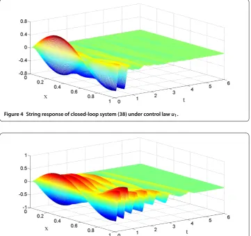
poly-Figure 4 String response of closed-loop system (38) under control lawu1.
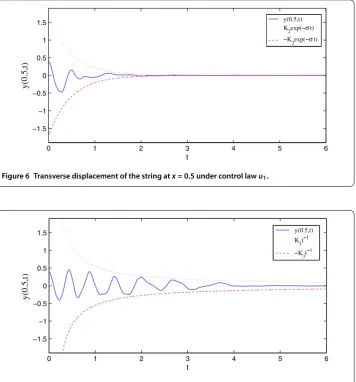
Figure 5 String response of closed-loop system (38) under control lawu2.
nomial decay with degree –, because r= ). The string responsey(x,t) of closed-loop system () with control lawuand control lawuare shown in Figure and Figure ,
respectively. The corresponding transversal displacement atx= . is shown in Figures and , respectively.
From Figures and , it can bee seen that, in the case of control lawu, the decay of the
transverse vibration relatively slow compared to the case of control lawu. Indeed, from
Figure and Figure , we know that in the case of control lawu, the transverse vibration
has been suppressed exponentially (|y(.,t)| ≤Ke–σt), whereas in the case of control
lawu, the transverse vibration has been suppressed polynomially (|y(.,t)| ≤Kt–). It
is coincident with the results of Theorem ..
Appendix
A.1 Proof of Lemma 3.1
Integrating by parts and () we get, for allt≥,
yx(x,t)yxt(x,t)dx=
yx(x,t)yt(x,t)
xdx–
yxx(x,t)yt(x,t)dx
=yx(,t)yt(,t) –
Figure 6 Transverse displacement of the string atx= 0.5 under control lawu1.
Figure 7 Transverse displacement of the string atx= 0.5 under control lawu2.
So we obtain equation (). Next, integrating by parts we compute
xyxyxxdx=
xyxxdx–
yxdx= y
x(,t) –
yxdx
for allt≥. That is, equation () holds. Finally, we write
xyxyttdx=
[xyxyt]tdx–
xytyxtdx ()
and
xytyxtdx=
xytxdx–
ytdx ()
A.2 Proof of Claim 1
Sincer> , hypothesis (H) implies
L|s|r≤u(s)≤L|s|
r if|s| ≤,
L|s| ≤u(s)≤L|s| if|s|> .
Hence, it is true that, for alls∈R,
s≤
–
L u(s)s
r+
–
L
u(s)s, ()
u(s)≤–Lru(s)s
r+–L
u(s)s. ()
Then, from () and Proposition . we have
S T
Eq(t)yt(,t)dt
≤
S T
Eq(t)
–
L
u(t)yt(,t)
r+
dt+
S T
Eq(t)
–
L
u(t)yt(,t)
dt
=
S T
Eq(t)
–E
(t)
L
r+
dt–
L
S T
Eq(t)E(t)dt
≤
S T
Eq(t)
–E
(t)
L
r+
dt+ E q+(T)
(q+ )L
. ()
From Young’s inequality, we have, for anyα,β,δ> ,
αβ≤δρα ρ
ρ +δ
–ρβ ρ
ρ, ()
whereρ,ρ> and ρ+ρ = . Applying the above inequality withα=Eq(t),β= (–E (t)
L ) r+, ρ=rr+–andρ=r+ , we obtain, for anyδ> ,
S T
E(t)q
–E
(t)
L
r+
dt
≤r–
r+ δ r+ r–
S T
Eqrr+–(t)dt+ δ
–r+
(r+ )L
S T
–E(t)dt
≤r–
r+ δ r+ r–
S T
Eqrr+–(t)dt+ δ
–r+
(r+ )L
E(T). ()
By inserting () into (), we deduce inequality () in Claim . Similarly, from () and Proposition . we have
S T
Eq(t)uyt(,t)
dt
≤ S T
Eq(t)–Lru(t)yt(,t)
r+dt+L
S T
Eq(t)–u(t)yt(,t)
=
S T
Eq(t)–LrE(t) r+dt–L
S T
Eq(t)E(t)dt
≤ S T
Eq(t)–LrE(t)r+ dt+ L (q+ )E
q+(T). ()
Applying again inequality () withα=Eq(t),β= [–Lr
E(t)]
r+,ρ=r+
r– andρ=
r+
, we
obtain, for anyδ>
S T
E(t)q–LrE(t) r+dt
≤r–
r+ δ r+ r–
S T
Eqrr+–(t)dt+L r
δ–
r+ (r+ )
S T
–E(t)dt
≤r–
r+ δ r+ r–
S T
Eqrr+–(t)dt+L r
δ–
r+
(r+ ) E(T). ()
Inserting () into (), we get inequality () in Claim .
Competing interests
The authors declare that they have no competing interests.
Authors’ contributions
All authors contributed equally to the manuscript and read and approved the final manuscript.
Author details
1Department of Mathematics, Harbin University of Science and Technology, Harbin, 150080, P.R. China.2Department of
Electronics Science and Technology, Harbin University of Science and Technology, Harbin, 150080, P.R. China.
Acknowledgements
This work is supported by the National Natural Science Foundation of China (Grant 11226128) and the Natural Science Foundation of Heilongjiang Province of China (Grant F201113).
Received: 22 April 2013 Accepted: 6 August 2013 Published: 21 October 2013 References
1. Chen, G, Delfour, MC, Krall, AM, Payre, G: Modeling, stabilization and control of serially connected beams. SIAM J. Control Optim.25, 526-546 (1987)
2. Lagnese, J: Decay of solutions of wave equations in a bounded domain with boundary dissipation. J. Differ. Equ.50, 163-182 (1983)
3. Shahruz, SM: Bounded-input bounded-output stability of a damped nonlinear string. IEEE Trans. Autom. Control41, 1179-1182 (1996)
4. Guo, BZ: Riesz basis approach to the stabilization of a flexible beam with a tip mass. SIAM J. Control Optim.39, 1736-1747 (2001)
5. Fung, RF, Wu, JW, Wu, SL: Exponential stabilization of an axially moving string by linear boundary feedback. Automatica35, 177-181 (1999)
6. Morgül, Ö: Stabilization disturbance rejection for the beam equation. IEEE Trans. Autom. Control46(12), 1913-1918 (2001)
7. Smyshlyaev, A, Guo, B-Z, Krstic, M: Arbitrary decay rate for Euler-Bernoulli beam by backstepping boundary feedback. IEEE Trans. Autom. Control54(5), 1134-1140 (2009)
8. Wang, JJ, Li, QH: Active vibration control methods of axially moving materials - a review. J. Vib. Control10, 475-491 (2004)
9. Luo, ZH, Guo, BZ, Morgül, Ö: Stability and Stabilization of Infinite Dimensional Systems with Applications. Communications and Control Engineering Series. Springer, London (1999)
10. Kirchhoff, G: Vorlesungen über Mechanik. Teubner, Stuttgart (1883)
11. Arosio, A, Panizzi, S: On the well-posedness of the Kirchhoff string. Trans. Am. Math. Soc.348(1), 305-330 (1996) 12. Ono, K: Global existence, decay, and blow up of solutions for some mildly degenerate nonlinear Kirchhoff strings.
J. Differ. Equ.137, 273-301 (1997)
13. Shahruz, SM, Krishna, LG: Boundary control of a non-linear string. J. Sound Vib.195, 169-174 (1996) 14. Oplinger, DW: Frequency response of a nonlinear stretched string. J. Acoust. Soc. Am.32, 1529-1538 (1960) 15. Wu, YH, Xue, XP, Shen, TL: Absolute stability of the Kirchhoff string with sector boundary control (under review) 16. Chen, G: Energy decay estimates and exact boundary value controllability for the wave equation in a bounded
domain. J. Math. Pures Appl.58, 249-273 (1979)
18. Lagnese, JE: Note on boundary stabilization of wave equations. SIAM J. Control Optim.26, 1250-1256 (1988) 19. Shahruz, MS: Suppression of vibration in a nonlinear axially moving string by boundary control. ASME Des. Eng. Tech.
Conf.106(1), 6-14 (1997)
20. Li, TC, Hou, ZC: Exponential stabilization of an axially moving string with geometrical nonlinearity by linear boundary feedback. J. Sound Vib.296, 861-870 (2006)
21. Kobayashi, T: Boundary position feedback control of Kirchhoff’s non-linear strings. Math. Methods Appl. Sci.27, 79-89 (2004)
22. Komornik, V: Exact Controllability and Stabilization. RAM: Research in Applied Mathematics. Masson, Paris; Wiley, Chichester (1994)
doi:10.1186/1687-2770-2013-215