R E S E A R C H
Open Access
Fundamental solution of the Laplacian on flat
tori and boundary value problems for the
planar Poisson equation in rectangles
Malik Mamode
**Correspondence:
[email protected] Laboratoire PIMENT, Université de la Réunion, Saint-Denis, 97400, Réunion, France
Abstract
The fundamental solution of the Laplacian on flat tori is obtained using Eisenstein’s approach to elliptic functions via infinite series over lattices in the complex plane. Most boundary value problems stated for the planar Poisson equation in a rectangle for which series-only representations of solution were known, may thus be solved explicitly in closed-form using the method of images. Moreover, the fundamental solution ofn-Laplacian on flat tori may also be simply derived by a convolution power.
PACS Codes: 02.30.Em; 02.30.Jr
Keywords: 2D Poisson equation; Green function; horizon; boundary value problem; flat torus; analytical solution
1 Introduction
The Poisson equation is certainly the simplest and the most famous partial differential equation of elliptic type which arises in many areas of mathematical physics, for example for steady state problems in electrostatics, heat conduction and fluid flow. The studies of boundary value problems (BVPs) for Poisson equation in finite or semi-infinite connected domains are ancient and well documented in many reference books [–]. Different analyt-ical methods to construct solutions of these problems exist such as separation of variables, eigenfunction expansion,etc.and may depend on the nature of boundary conditions and the shape of domains. Among these methods, the method of source function, also called the Green function method, is the only one giving convenient and compact analytical rep-resentation of solutions in two- or three-dimensional space. In this method, the BVPs are reformulated into integral equations that involve the boundary conditions and the related Green function. But, as is well known, the actual implementation of the source function method in applications is often intricate owing to the difficulty to obtain a closed-form an-alytical expression for the Green function. This is notably the case for the BVPs for Poisson equation in rectangular domains for which series-only representations of Green functions are used [], although it is possible in principle to circumvent the difficulty by converting known closed-form results obtained for half-plane or circular domain into the rectangle via conformal transformations. Thus, using a conformal Schwarz-Christoffel transforma-tion mapping the half-plane into the rectangle, one can easily find the closed-form solutransforma-tion of homogeneous Dirichlet problem in terms of Jacobi elliptic functions (see for instance
[, , ]), but to date a large number of other BVPs for rectangular Poisson equation still have no analytical closed-form solutions.
We show in the present paper that the solutions of these BVPs amount to solve the Poisson equation on flat tori in the distributional sensei.e.in the space of doubly periodic Schwartz distributions on the Euclidean planeE=RorC[, ]. For this, the funda-mental solution of the Laplacian is first obtained in Section in terms of elliptic functions using Eisenstein’s approach via infinite series over rectangular lattices inC. Secondly, us-ing the method of images for instance, the analytical closed-form representation of Green functions for most BVPs stated for planar Poisson equation in the rectangle may easily be derived as shown in Section .
2 Fundamental solution and concept of horizon
Most BVPs for rectangular Poisson equation may reduce to solve in a distributional sense an equation of the formV=FonE, where the boundary conditions act as source terms and appear in the RHS of the equation. In particular, the equation
G=∂ G
∂x +
∂G
∂y =δ(x,y), (x,y)∈R
, ()
whereδ(x,y) is the Dirac distribution at origin, defines the so-called fundamental solution for the Laplacian on the plane. But, as is well known, the solution of () is not unique since given the particular solutionlog(x+y)/π, all solutions of () must be written of the form
G(x,y) = πlog
x+y+h(x,y),
wherehis an arbitrary harmonic function inR i.e.a solution ofh= . Nevertheless, the fundamental solution is that for which it is usually seth= constant and this may be justified in a heuristic manner as follows. Equation () may be seen as establishing a causal connection between a point source located at the origin, and the change produced at point (x,y) to a certain propertyGof the free space. In that sense, in the absence of source, this spatial property governed by () does not change and has to remain uniform:h= thus must necessarily implyh= constant. In addition, since the fundamental solution may also reflect some geometrical properties of the space like isotropy, it must possess circular symmetryi.e.must depend only on one variabler=x+yand it is easy to show that the only harmonic functions with circular symmetry are again constant functions.
Thus, all these reasons lead us to define the fundamental solution of Laplace equation onEas follows:
G(x,y) = πlog
x+y r
, ()
horizon (which may be chosen as far as wanted) restores the property thatGtends to as (x+y)/→rwhich is, here at finite distance, the property retained for the fundamental solution of Laplace equation in (n> )-dimensional space for which the horizon is located at infinity.
In this cause-and-effect relationship, the distribution solutionV∈D(R) of BVPs may be readily obtained by ‘division’i.e.may be given by the double convolution product,
V=G∗x∗yF= πlog
x+y r
x ∗∗yF.
Thus, by a such algebraic approach, the existence of the solution is simply related to the existence of the convolution product inD(R) hence the causal solution is derivedup to a constantprovided that
+∞
–∞ dξ
+∞
–∞ dηF(ξ,η) < +∞. ()
We focus our attention in the rest of this note to the case where the source termFis doubly periodic in thex,y-variables. We shall see indeed that the BVPs for the rectangle, not surprisingly, are relevant to that case related to the tessellation of the Euclidean plane
Ewith an infinite number of identical rectangular tiles in bothx,y-directions.
Assume thatFis of period aand b in thex- andy-variable, respectively. It is thus always possible to define the distributionFon the rectangle{(x,y)|–a<x<a, –b<y<b} such that ‘by gluing together the pieces’ []
F(x,y) = +∞
n=–∞ +∞
m=–∞
δ(x– na)δ(y– mb)∗x∗yF(x,y).
The distributionFis thereby biunivocally associated toF∈D(R) and it is a distribution on the flat torus a,b=E/a,b, quotient of the Euclidean plane by the latticea,b= aZ+
ibZ. In order that the condition () holds, it is here necessary to prescribe the following compatibility condition:
a
–a
dξ
b
–b
dηF(ξ,η) = , ()
so that the solution of the Poisson equationV=F, initially posed onE, is the (doubly periodic) distribution on a,bformally expressed as the convolution product on the torus,
V=a,b(x,y) x
∗∗yF(x,y), ()
where
a,b(x,y) =
+∞
n=–∞ +∞
m=–∞
δ(x– na)δ(y– mb)∗x∗yG
= π
+∞
n=–∞ +∞
m=–∞
log (x– na)
+ (y– mb)
r
= πlog
+∞
n=–∞ +∞
m=–∞
(x– na)+ (y– mb) r
provided that the previous series is convergent,which is unfortunately not the case for any fixed r.
To overcome this difficulty, let us notice that the solutionVshould be unchanged owing to the compatibility condition (), if the termr
is replaced by
rnm= na+ mb for|n|+|m| = ()
(the nonzero termris not specified, as its value is not essential due to the compatibility condition ()). In other words, the horizon of (n,m)th term of the series is not at all taken constant but is assumed to correspond to the distance from the center of rectangular tile
{(n– )a<x< (n+ )a, (m– )b<y< (m+ )b}to the originviz.the center of funda-mental rectangle. In this way, it follows that the double infinite product () may be seen as the modulus square of
φ(z) = z r
+∞
n=–∞ +∞
m=–∞
+ z
na+imb
, z=x+iy, ()
where the dash, as is customary, denotes omission of the term inn=m= . Nevertheless, the product ()is always not absolutely convergentand has not the rearrangement prop-ertyi.e.its limitφ(z) (if it exists) is dependent of the order of the factors. Using thus the Eisenstein convention [] which groups together the factors of opposite rank according to the following calculation process:
lim
M→+∞
+M
m=–M lim
N→+∞
+N
n=–N
(the order of limits is imposed; see []), the specific result denotedφe(z) becomes an entire
function having zeros only at points of the latticea,bbut is not doubly periodic in virtue
of Liouville’s theorem despite appearances. Indeed, using the Eisenstein convention, () shows at once thatφe(z+ a) = –φe(z) and soφe has period a, while under translation
along the imaginary axis,
φe(z+ ib) = –eπb/ae–iπz/aφe(z). ()
See [] for a proof. Hence, following Eisenstein’s approach to elliptic functions via infinite series over lattices inC[], we may write
φe(z)∝ϑ
πz a
ib
a
,
whereϑdenotes the first Jacobi theta function []. At this point, it is no longer difficult to show that the convolution kernela,b,up to a constant, is thus explicitly given by
a,b(x,y) =
πlog e
–πy/ab
ϑ
π
a(x+iy)
ib
a
Indeed, firstlya,b∈D( a,b) and the double periodicity is recovered due to the
exponen-tial term since by (),
a,b(x,y+ b) =
πlog
e–π(y+b)/abφe(z+ ib)
= πlog
e–πy/abφe(z)=a,b(x,y).
Secondly, it can be proved that
a,b=δ(x)δ(y) –
ab ()
on the flat torus a,bi.e.a,bis the fundamental solution (Green function) for the
Lapla-cian on a,b. Indeed,φe(z) is zero atz= so thata,bhas a singularity at the center of
the torus and,
a,b+
ab=
∂
∂z∂zlogφe(z) = forz=
(here and in the sequel, the principal branch of the logarithm is considered). In addition, applying the Green theorem on a fundamental domain of the torus,
a,b
a,b+
ab
dx dy= π
a,b
logφe(z)dx dy
= π
∂ a,b
∂
∂zlogφe(z)dz.
Since
∂
∂zlogφe(z) =
π
a d dwlogϑ
wib a
=ζ(z) –ζ(a)
a z withw=
πz a,
ζ(z) being theζ-Weierstrass elliptic function, which is meromorphic, having a simple pole at the origin (and no others on the integration domain) with residue [], it follows from the residue theorem that
a,b
a,b+
ab
dx dy= π
∂ a,b
ζ(z) –ζ(a) a z
dz= .
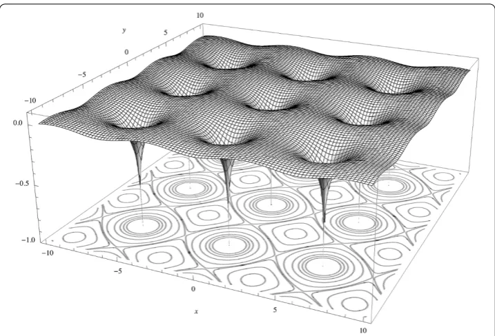
This completes the proof. A surface plot of the fundamental solutiona,bis given in
Fig-ure fora=b= .
Remarks (i) Let us notice that interchanging the roles of variablesxandyin what pre-cedes yields an equivalent formulation of the fundamental solution,
a,b(x,y) =
πlog e
–πx/abϑ
π
b(y+ix)
ia
b
, ()
or in a more symmetrical form,
a,b(x,y) =
πlog e
–π(x+y)/ab
ϑ
π
a(x+iy)
ib a ϑ π
b(y+ix)
ia
b
Figure 1 Relief of the fundamental solutiona,b(x,y) on the flat torusa,bfora=b= 3 (shown over nine fundamental domains of the torus), and equipotential linesa,b(x,y) =constant.
(ii) Since from (),
(a,b x
∗∗ya,b) =a,b x ∗∗ya,b
=
δ(x)δ(y) – ab
x ∗∗y
δ(x)δ(y) – ab
=δ(x)δ(y) – ab,
it follows by induction that, for any integern≥,
n(a,b x
∗∗ · · ·y ∗x∗ya,b
n
) =na∗,nb=δ(x)δ(y) – ab,
which shows that the convolution powera∗,nb(x,y) is the fundamental solution for the (n≥ )-Laplacian on the flat torus a,b.
3 Applications
Having found the fundamental solution for the Laplacian (), it is straightforward us-ing the image method (by an appropriate periodic distribution of images) to obtain the exact expression of the Green function for most BVPs stated for Poisson equation in the rectangle.
Thus, for the Dirichlet problem, the related Green functionGD(x,y;x,y)i.e.the solu-tion of the equasolu-tionGD=δ(x–x)δ(y–y) on the rectangle{(x,y)| <x<a, <y<b}
distri-bution solution of
GD=δ(x–x)δ(y–y) –δ(x+x)δ(y–y) –δ(x–x)δ(y+y) +δ(x+x)δ(y+y)
on the flat torus a,b(note that the compatibility condition () is well fulfilled) is simply
given by
GD(x,y;x,y) =a,b(x–x,y–y) –a,b(x+x,y–y)
–a,b(x–x,y+y) +a,b(x+x,y+y),
i.e.by settingz=x+iyandz=x+iy,
GD(x,y;x,y) =
π log
ϑ(πa(z–z)|iab)ϑ(πa(z+z)|iba)
ϑ(πa(z+z)|iba)ϑ(πa(z–z)|iba)
. ()
This result is to be compared with that obtained in []. Here, it is worth to note that in addition to its simplicity, the complex formulation of the Green function together with the properties of functions of a complex variable and of conformal transformation may provide us with several methods for extending as desired the Dirichlet problem to many other geometries [].
Similarly, for the Neumann problem, the ‘generalized Green function’ (also called Neumann function)GN(x,y;x,y)i.e.the solution of the equationGN =δ(x–x)δ(y–
y) – ab on the rectangle{(x,y)| <x<a, <y<b}with the homogeneous conditions
∂GN
∂n = on the sides (∂/∂ndenotes as usual the outward normal derivative; notice that
here the compatibility condition () is nothing but the Gauss theorem), or equivalently the periodic distribution solution of
GN=δ(x–x)δ(y–y) +δ(x+x)δ(y–y) +δ(x–x)δ(y+y)
+δ(x+x)δ(y+y) – ab
on the flat torus a,bis thus given by
GN(x,y;x,y) =a,b(x–x,y–y) +a,b(x+x,y–y)
+a,b(x–x,y+y) +a,b(x+x,y+y),
i.e.
GN(x,y;x,y) = –
y+y ab +
π log ϑ
π
a(z–z)
ib
a
ϑ
π
a(z+z)
ib
a
×ϑ
π
a(z+z)
ib
a
ϑ
π
a(z–z)
ib
a
. ()
To illustrate the practical value of such an analytical result, consider the Poisson equation
u=f(x,y) on the unit square{ <x,y< }subject to homogeneous Neumann boundary conditions and where
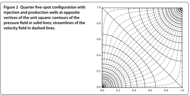
Figure 2 Quarter five-spot configuration with injection and production wells at opposite vertices of the unit square: contours of the pressure field in solid lines; streamlines of the velocity field in dashed lines.
models two unit points sources of opposite strength and located on a diagonal of the square. The solution is at once given up to a constant by
u(x,y) =
dξ
dηGN(x,y;ξ,η)f(ξ,η)
=GN(x,y;ε,ε) –GN(x,y; –ε, –ε)
and, taking the limitε→, the result obtained after simplification,
u(x,y) =
π log
ϑ(πz|i)
ϑ(πz|i)
, z=x+iy ()
may be considered as the exact analytical solution of a standard porous media problem known as the homogeneous quarter five-spot problem which is a popular test case sce-nario in oil reservoir simulation []. Figure shows the contours of the pressure field () and the streamlines of the velocity field defined by the curves
log ϑ( π
z|i)
ϑ(πz|i)
= constant,
which agree well with numerical simulations [].
4 Perspectives and conclusions
number of problems posed on regions of more complicated shape and with a mixed set-ting of different kinds of boundary conditions. Although it was not the primary object of this note, having obtained the fundamental solution ofn-Laplacian on the flat torus will also be of great interest for explicitly solving BVPs for two-dimensionaln-harmonic equa-tion in rectangles as, for instance, the biharmonic equaequa-tion and the linear clamped plate boundary value problem in mechanics.
Competing interests
The author declares that he has no competing interests.
Acknowledgements
The author would like to thank the referees for their valuable remarks and suggestions.
Received: 11 July 2014 Accepted: 16 September 2014
References
1. Morse, PM, Feshbach, H: Methods of Theoretical Physics, vol. 1. McGraw-Hill, New York (1953) 2. Morse, PM, Feshbach, H: Methods of Theoretical Physics, vol. 2. McGraw-Hill, New York (1953) 3. Tikhonov, AN, Samarskii, AA: Equations of Mathematical Physics. Dover, New York (1990)
4. Melnikov, YA, Melnikov, MY: Computability of series representations for Green’s functions in a rectangle. Eng. Anal. Bound. Elem.30, 774-780 (2006)
5. Shou, Q, Jiang, Q, Guo, Q: The closed-form solution for the 2D Poisson equation with a rectangular boundary. J. Phys. A, Math. Theor.42, 205202 (2009)
6. Gel’fand, IM, Shilov, GE: Generalized Functions, vol. I. Academic Press, New York (1964) 7. Schwartz, L: Mathematics for the Physical Sciences. Addison-Wesley, Reading (1966) 8. Walker, PL: Elliptic Functions: A Constructive Approach. Wiley, New York (1996)
9. Gradshteyn, IS, Ryzhik, IM: Table of Integrals, Series and Products. Academic Press, New York (2000)
10. Driscoll, TA, Trefethen, LN: Schwarz-Christoffel Mapping. Cambridge Monographs on Applied and Computational Mathematics, vol. 8. Cambridge University Press, Cambridge (2002)
11. Chen, CY, Meiburg, E: Miscible porous media displacements in the quarter five-spot configuration. Part 1. The homogeneous case. J. Fluid Mech.371, 233-268 (1998)
doi:10.1186/s13661-014-0221-4