Practical design of delta-sigma multiple description audio coding

R E S E A R C H

Open Access

Practical design of delta-sigma multiple

description audio coding

Jack Leegaard

, Jan Østergaard

, Søren Holdt Jensen

and Ram Zamir

Abstract

It was recently shown that delta-sigma quantization (DSQ) can be used for optimal multiple description (MD) coding of Gaussian sources. The DSQ scheme combined oversampling, prediction, and noise-shaping in order to trade off side distortion for central distortion in MD coding. It was shown that asymptotically in the dimensions of the resampling, prediction, and noise-shaping filters as well as asymptotically in the quantizer dimensions, all rate-distortion points on the symmetric quadratic Gaussian MD rate-distortion function could be achieved. In this work, we show that this somewhat theoretical framework is suitable for practical low-delay MD audio coding. In particular, we design a practical MD audio coder with two descriptions and provide simulations on real audio data. The simulations demonstrate that even when using low-dimensional noise-shaping, prediction, and resampling filters, it is possible to obtain good quality audio in the presence of packet losses. Simulations on real audio reveal that, contrary to existing designs, it is straightforward to obtain a large number of trade-off points between side distortion and central distortion, which makes the proposed coder suitable for a wide range of applications.

Keywords: Audio coding; Multiple descriptions; Noise shaping; Predictive coding

1 Introduction

There is a growing interest in achieving reliable stream-ing of high-quality audio over networks for digital audio broadcast services, internet radio, youtube, and similar multimedia streaming services. High-quality streaming can be achieved by using, e.g., error-correcting codes and by allowing large delays, large bandwidths, or dedi-cated/prioritized networks. However, for certain applica-tions, long delays cannot be tolerated. For example, for interactive services such as voice over IP or musicians playing together via the internet, it is crucial that the delay is kept at a minimum. Indeed, for the latter case, it has been noted that delays less than 5 ms are often required [1].

Conventional broadband connections in homes are generally asymmetric in the sense that their downlink capacity is much greater than their corresponding uplink capacity. While this is good for common internet usage such as browsing, it is not ideal for interactive

high-*Correspondence: [email protected]

1Department of Electronic Systems, Aalborg University, Niels Jernes Vej 12, Aalborg 9220, Denmark

Full list of author information is available at the end of the article

quality streaming services, where instead a more sym-metric strategy would be advantageous. To reduce the required bandwidth for audio streaming services, it is common to exploit efficient audio compression methods. Thede factostandard for lossy compression of music is the family of advanced audio coding (AAC) algorithms, which have been standardized by ISO and IEC as part of the MPEG-2 and MPEG-4 specifications [2-4]. AAC is used for audio compression for digital TV as well as digital audio broadcast (DAB) in several countries. AAC achieves better quality than MP3 and allows for high sampling rates and multiple channels [5]. It is based on the modified dis-crete cosine transform (MDCT), which is able to provide a high-frequency resolution by using long delays [5]. For low-delay coding, transform coders are generally not as efficient as parametric (model based) coders [6]. Recently, low-delay parametric audio coders based on linear predic-tion [6,7] and generalized noise-shaped quantizapredic-tion [8] have been proposed. With such techniques, it is possible to achieve delays less than 5 ms while maintaining high-quality audio. In fact, even a few sample delays can be achieved by compromising the efficiency of the perceptual model [6-8].

In order to achieve a certain degree of robustness towards packet dropouts or channel failures, it is possi-ble to use error-correcting codes. If the tolerapossi-ble delay or bandwidth is large enough, then these codes can be extremely efficient. An alternative is to use joint source-channel coding techniques, where a certain amount of source redundancy is introduced to help the chan-nel/source decoder at the receiving end. A particular case is multiple description (MD) coding [9], where the source is encoded into multiple (partially) redundant packets, which can be decoded independently of each other. More-over, if several packets are received, then they are able to refine each other and, thus, improve the reconstruc-tion quality. MDs generalize the concepts of repetireconstruc-tion coding and layered source coding (i.e., successive refine-ments), where in the former case, a packet is simply duplicated, and in the latter case, packets are (nearly) independent of each othera_{. In [10], it was shown that a}

tolerable music quality could be achieved even on unreli-able networks having more than 30% packet dropouts by using MDs audio coding between two and four descrip-tions (packets). The MD audio coding schemes pre-sented in [10] and [11] are both based on transform coders and therefore not able to achieve ultra low delay. Recently, a predictive strategy for high-quality audio MD coding was presented in [12] and a noise-shaped strat-egy in [8], which are both able to achieve very low delays.

Common for existing MD audio coders are that the audio coding part and the MD part are somewhat sepa-rated and only a few trade-off points on the operational MD rate-distortion function can be obtained. On the other hand, in this paper, we use a unified strategy based on predictive coding and noise shaping that allows an almost continuous trade-off between rate and distortions of the descriptions. In particular, in [13], an inherent connection between oversampled delta-sigma quantization

and MD coding for Gaussian sources was discovered. By oversampling the signal, a certain amount of redun-dancy is introduced, and by proper noise shaping of the quantization noise a trade-off between the reconstruction qualities due to receiving different subsets of descriptions is possible, cf. Figure 1. The work in [13] treated white Gaussian signals and noise shaping and was extended to the case of predictive coding and noise shaping of colored Gaussian sources in [14,15].

In this paper, we construct an efficient high-quality low-delay MD coder based on the principles of oversampling, predictive coding, and noise shaping. Specifically, we uti-lize the theoretic construction proposed for Gaussian sources in [13-15] and show that it naturally extends to real audio signals. We restrict attention to two descrip-tions and a symmetric setup, where the rate-distortion performance of the individual descriptions are identi-cal. It is worth emphasizing that contrary to Gaussian source coding, it is crucial in audio coding that the tem-poral envelope is kept smooth when filter parameters are updated. This complicates the transition from theory to practice. The contributions of this paper are there-fore dedicated to the practical design of the coder, and we refer the reader to the aforementioned literature for the theoretical foundations. The present paper discusses the design of filters for resampling, prediction, and noise shaping, in addition to coding the parametersb. The pro-posed design is evaluated on several audio signals sampled at 48 kHz, and the performance due to receiving different subsets of descriptions is assessed. Moreover, the pro-posed coder is simulated in an environment with packet losses. It is shown that good quality music is achievable with delays less than 5 ms.

In comparison, the low-delay noise-shaped coder in [8] reveals a significant reduction of the coding rate, which is mainly due to the inclusion of individual description prediction loops.

2 Background

The MD predictive noise-shaped coder proposed in [13-15] consists of sampling rate conversion, encoders, noise-shaping, and decoding. We briefly describe these components below and refer to [13-15] for further details.

2.1 Sampling rate conversion

In the MD noise-shaped predictive coder proposed in [13-15], the original signalx(n)is first oversampled by a factor of two to obtainxup(m)as shown in Figure 1. We

use the indicesnandmto refer to samples of signals in the original and upsampled domains, respectively. Sam-pling rate conversion of discrete-time audio signals has been widely studied in the audio engineering literature, cf. [16-18] to name a few. Theoretically, if the signal is ban-dlimited, then changing its sampling rate is a reversible process, as long as the resulting sample rate is greater than the Nyquist frequency of the signal, i.e., greater than twice the signals’ bandwidth.

2.2 Encoder

The upsampled signal is split into even and odd sam-ples (see Figure 1), and the even (odd) stream is fed to the even (odd) encoder. Each encoder can be cast in the framework of ‘noisy’ single-description prediction, which in case of Gaussian signals was treated in [19]. In [19], it was shown that optimal encoding is achieved with mini-mum mean square error (MMSE) prediction. This result was used in [14] to show that the optimal encoders should be MMSE prediction filters for the colored ‘even’ and ‘odd’ Gaussian signals, respectively. Interestingly, in [15], it was furthermore suggested that the encoders could actually be any existing standard compression schemes. Indeed, in [20], it was proposed to combine delta-sigma quantization with standard JPEG coding schemes to form compres-sion algorithms for MD coding of still images. Similarly, in this work, we could choose to use e.g., standard AAC compression schemes. A key motivation for choosing a standard coder is of course the fact that one avoids the trouble of having to design an efficient audio coder, but perhaps more interestingly, the individual descriptions would then also be completely standard-compliant with existing technology. Only if both descriptions are to be jointly considered at the receiving end, the decoder needs to be slightly altered.

2.3 Noise shaping

We now turn our attention to the feedback filter whose purpose is to perform noise-shaping of the coding noise [21]. As illustrated in Figure 1, the coding noiseseeven(n)

andeodd(n)from the two encoders are interlaced to form

the error signale(m)having the same sampling frequency asxup(m). The error signale(m)is filtered by the

noise-shaping filter and then added to xup(m) and thereby

closing the feedback loop. The purpose of the noise-shaping filter in conventional oversampled quantization (e.g., delta-sigma quantization) is to shape the noise away from the in-band spectrum and thereby reduce the energy of the noise, which is imposed upon the signal [21]. In MD coding, on the other hand, the purpose is to shape the noise so that a proper trade-off is achieved regarding the distortion due to receiving a single packet versus receiv-ing both packets [13]. Indeed, it is illustrative to consider what happens when only a single packet is received. In this case, since we split the signal into even and odd samples, we have in fact downsampled the oversampled signal by a factor of two (without first applying an anti-aliasing filter). But since the source spectrum only covers half the fre-quency spectrum ofxup(m)(due to oversampling), there

will not be any source aliasing. On the other hand, due to interlacing the noise samples, the noise spectrum cov-ers the full frequency range, see Figures Eight and Twelve in [13] for an illustration of the noise spectra. Thus, the noise spectrum will be aliased. In particular, the out-of-band noise spectrum will be aliased and superimposed upon the in-band source + noise spectrum. The effect is that no matter how the noise is shaped, the full noise spec-trum will be imposed upon the source specspec-trum. On the other hand, if both packets are received, the oversampled signal can be recovered without noise aliasing and, thus, it is possible to apply a low-pass filter and get rid of the out-of-band noise. To summarize, on one hand, we would like to minimize the total noise energy in order to reduce the distortion when receiving only a single packet. On the other hand, we would like to put as much noise in the high-frequency spectrum and thereby reduce the amount of noise in the in-band spectrum, in order to minimize the distortion when receiving both packets. It is also interest-ing to note that the entropy rate of the quantizer, under high-resolution conditions, is independent of the noise-shaping filter and given by the ratio of the powerσ_X2 of the input signal and the power of the excitation noise (the inpute(m)to the noise-shaping filter), i.e.,

R≈ 1

2log2

σ_X2 σ2 e

.

2.4 Decoder

At the receiver, the received signals are decoded as shown in Figure 2. If only a single packet is received, the corre-sponding decoder is applied. If both packets are received, the even and odd signals are first individually recon-structed and then interlaced to form an approximation ofxup(m). Then, a low-pass filter is applied to get rid of

Figure 2Schematics of the MD noise-shaped predictive decoder [13-15].

3 Practical construction of the MD audio coder

In the following subsections, the design of the individual parts of the coder is described.

3.1 Sampling rate conversion

Ideal oversampling can theoretically be obtained by inserting zeros between every sample of the original signal and then apply an ideal low-pass filter (i.e., convolution by an infinite-length sinc function). The resulting signal xup(m)has twice as many samples asx(n), and form=2n

andm even, we have thatxup(m) = x(n) (if we ignore

possible integer time-delays due to filtering). Thus, we recover the original signal simply by taking all the even samples ofxup(m). The odd samples ofxup(m)are

phase-shifted versions ofx(n). Of course, in practice, we cannot use ideal low-pass filtering since this will result in pro-hibitively large delays. Due to using finite filters, a certain degree of aliasing is unavoidable.

In this work, we use an FIR filterh(z)with linear phase obtained via the window method (Chebyshev) as the inter-polation filter [22]. Specifically, we insert zeros between every sample of x(n) and apply the filter to obtain the upsampled signal xup(m) [16]. Figure 3 shows the

per-formance in MSE as a function of the filter length. The

Figure 3Error due to resampling using finite length filters.

solid lines are for a unit-variance audio signal ‘Abba’cand the dashed lines (with circles) are for a zero-mean unit-variance white Gaussian signal. As foreshadowed above, the error on the even samples due to resampling is negli-gible for filter orders greater thanN = 18. On the other hand, the odd samples are highly affected by the resam-pling operation, which is due to frequency aliasingd. An estimate of the power spectral density (PSD) of the Abba signal is shown in Figure 4. It is clear that it is not flat, and, thus, the impact of aliasing is much less than for the Gaussian case.

3.2 Closed-loop prediction

Let us momentarily forget about the feedback loop shown in Figure 1 (since this will be treated in the following sub-section) and simply consider thatxup(m)is to be split into

its even and odd samples, which are denoted byzeven(n)

and zodd(n) in Figure 1. For clarity, we have redrawn

the encoder with more details in Figure 5. The even sig-nal zeven(n) is now fed into a compression algorithm

(encoder), and the compressed signalyeven(n)is

transmit-ted to the decoder. The odd signalzodd(n)is processed in

Figure 5Schematics of the complete MD noise-shaped predictive encoder [14,15].

a similar way. Thus, the even samples then constitute one of the packets in the MD coder, and the odd samples con-stitute the other packet. The number of samples to include in each packet depends upon several factors and will be treated in the sequel.

3.2.1 Linear predictive coding

The encoders will in this work be given by forward lin-ear prediction coding. In particular, in order to encode the even signalzeven(n), we design a linear predictor based on

the even unquantized sampleszeven(n). We use a forward

linear predictor, which as usual is obtained by minimiz-ing the prediction error in the least squares sense, cf. [23] for details. The predictor performs closed-loop predic-tion, i.e., the quantizer is contained within the prediction loop [19]. To do so, we consider a block of samples and use these for estimating the prediction filter. The filter needs to be encoded and transmitted to the decoder. Thus, there is a trade-off between the rate required for coding the filter coefficients, the update rate of the filter, and the rate required for coding the prediction error. A general approach to choosing a proper rate distribution between model parameters and signal was considered in [24].

3.2.2 Coding the prediction error

Even though the prediction filters are updated only once per block of samples, quantization of the prediction error is performed on a sample-by-sample basis. Thus, we need to use scalar quantization, and for simplicity, we will use scalar uniform quantization [25]. We therefore only need to design the proper step-size of the quantizer. To obtain the bitrates of the coder, we first run the predic-tor using a fixed step sizeon a large data set of mixed audio having a sampling frequency of 48 kHz. Then, a scalar (Huffman) entropy coder is designed on the quan-tized output of the predictor [26]. Thus, we are using a

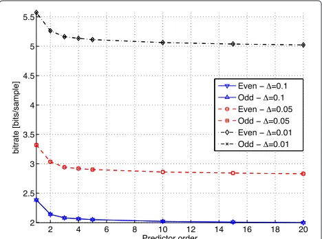
static and memoryless entropy coder. Finally, the predic-tor is tested on an audio segment (in this case, it consists of jazz music), which is not part of the training material. Figure 6 shows the resulting coding rate due to using a scalar uniform quantizer with a step-sizefollowed by a scalar (Huffman) entropy coder. The corresponding MSE due to changing the step size of the quantizer is shown in Figure 7. In these simulations, we update the two lin-ear predictive coding (LPC) filters once in each block of 128 samples. Since the audio signals have a sampling fre-quency of 48 khz, then if the bitrate is say 5 bits/sample, the resulting rate for coding the prediction error is 240 kbps per packet.

3.2.3 Predictor order

In predictive audio coding, it is common to use predictors of orders greater than 10 [6]. However, in our case, the

Figure 7MSE due to forward linear prediction and encoding the prediction error.

outer loop introduces noisy feedback, which to a certain degree reduces the predictor capabilities. For example, let = 0.01, and construct a 10th-order noise-shaping fil-ter using the design in Equation 1 provided in the next subsection. Then, the performance in terms of rate and distortion of the predictor as a function of its order is shown in Figures 6 and 7. The bitrates illustrated in the figures correspond to the rates required for encoding the prediction residuals. The actual predictor coefficients have not been coded in these simulations. The simulations are repeated for a wide range of predictor orders. It may be noticed that increasing the order from 1 to 5 significantly decreases the required bitrate for coding the residual, whereas using an order above 10 does not lead to signifi-cant improvements. On the other hand, the resulting MSE is approximately unaffected by the predictor order.

3.3 Noise shaping

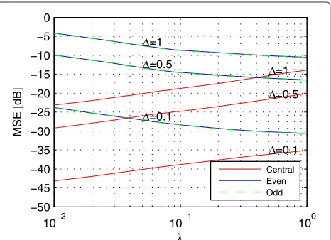
The purpose of the noise-shaping filter is to shape the quantization noise appropriately in the frequency domain [21]. Ideally, the frequency response of the noise-shaping filter should be a two-step function, which in the in-band frequency range has power δ−1 and in the out-of-band frequency range has powerδ [13]. Thus, if both descrip-tions are received, one is able to filter out the out-of-band noise and thereby obtain a resulting noise power that is proportional to δ−1. On the other hand, if only a single description is received, then due to aliasing, the resulting noise power is proportional toδ+δ−1. Furthermore, fix-ing the levels asδ andδ−1, respectively, guarantees that their geometric mean is one, which basically fixes the cod-ing rate while allowcod-ing one to trade-off side distortion for central distortion [13].

In practice, we need to approximate the two-step response using a finite length feedback filter. The optimal

design of the noise-shaping filterc(z)for any filter orderp was given in [13] as:

c= −(G+2λI)−1g (1) where c = (c1,. . .,cp)T are the filter coefficients, g =

(sinc(1/2), sinc(2/2),. . ., sinc(p/2))T, andGis the matrix with entriesGi,j = sinc((i−j)/2),i,j = 1,. . .,p. In (1),

λdenotes the trade-off between central and side distor-tion. Choosingλ = 1 indicates that the central and side distortion are given the same weight. In this case, the cen-tral distortion will on average be around 3 dB smaller than the side distortion. On the other hand, choosing λ 1 reduces the central distortion at the price of increasing the side distortion. This is illustrated in Figures 8 and 9 for the case ofp = 10 andp = 30, respectively. In these simu-lations,∈ {0.01, 0.05, 0.1}. It may be noticed that larger yields larger distortions as expected. It can also be seen that for large λ, the central distortion is approximately −10 log₁₀(λ)dB smaller than the side distortion.

3.3.1 Coding the predictor coefficients

There exists a vast amount of literature on efficient encod-ing of LPC coefficients, cf. [27] and the references therein. Here, we will use a common approach and transform the LPC coefficients to line spectral frequencies (LSF) coef-ficients [28]. This is done partly due to the fact that it is easy to guarantee stability of the inverse filter in the LSF domain and partly due to fact that they are easier to encode efficiently [29]. From Figure 6, it is clear that using a filter order above 10 does not significantly decrease the coding rate for the prediction error over what is possible with a 10th order filter. We therefore proceed using a 10th order predictor, which is first converted to 10 LSF coeffi-cients. The 10 LSF coefficients are then quantized using a scalar quantizer with a step size ofπ/64. The quantized coefficients are then split into three subvectors of length

10−2 10−1 100

−50 −45 −40 −35 −30 −25 −20 −15 −10 −5 0

λ

MSE [dB]

Δ=0.1

Δ=0.5

Δ=1

Δ=0.1

Δ=0.5

Δ=1

Central Even Odd

10−2 10−1 100 −50

−45 −40 −35 −30 −25 −20 −15 −10 −5 0

λ

MSE [dB]

Δ=0.1 Δ=0.5 Δ=1

Δ=0.1 Δ=0.5 Δ=1

Central Even Odd

Figure 9Performance for the Abba signal when using a noise shaping filter of orderp=30.

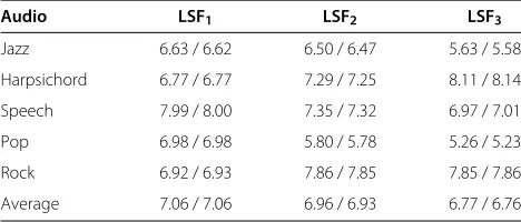
3, 3, and 4, respectively. Finally, each subvector is inde-pendently vector Huffman coded. The resulting bitrates are shown in Tables 1 and 2, where LSFidenotes theith

subvector. In these simulations, the window size of the predictor is 128 samples. It may be noticed from Table 2 that the average coding rate is approximately 20.8 bits per LSF vector. Since the sampling frequency is 48 kHz and the block size is 128 samples, the resulting average bitrate for coding the LSF vectors is 7.8 kbps per packet.

3.4 Decoding

Decoding the received audio packets is more challenging than in conventional audio coding since the encoder does not know which packets (if any) the decoder receives. In fact, since the encoder forms two packets, the decoder will at each time instance enter one of 16 different states, which depends upon its previous state, see Table 3. If the decoder remains in one of the states on the ‘diagonal’ in Table 3, i.e., states 1, 6, 11, or 16, it is straightforward to guarantee a smooth transition between blocks. The prob-lem occurs when the decoder switches to the other states. We solve these issues in the sequel.

Table 1 Bitrates for coding the (even/odd) subvectors of the LSF vector

Audio LSF1 LSF2 LSF3

Jazz 6.63 / 6.62 6.50 / 6.47 5.63 / 5.58

Harpsichord 6.77 / 6.77 7.29 / 7.25 8.11 / 8.14

Speech 7.99 / 8.00 7.35 / 7.32 6.97 / 7.01

Pop 6.98 / 6.98 5.80 / 5.78 5.26 / 5.23

Rock 6.92 / 6.93 7.86 / 7.85 7.85 / 7.86

Average 7.06 / 7.06 6.96 / 6.93 6.77 / 6.76

LSFidenotes theith subvector.

Table 2 Bitrates (in bits/vector) for coding the (even/odd) LSF vectors

Audio LSF vector

Jazz 18.76 / 18.67

Harpsichord 22.17 / 22.17

Speech 22.32 / 22.33

Pop 18.04 / 17.99

Rock 22.64 / 22.63

Average 20.79 / 20.76

3.4.1 State 1

This is the case with no packet dropouts. The decoder simply processes the two descriptions as described in Subsection 2.4. Both descriptions are first individually reconstructed, then interlaced, and finally downsampled to produce a single high-quality reconstruction. Thus, the states of the LPC filters at the side decoders as well as the state of the low-pass filter at the central decoder are all properly updated, which results in smooth transitions between consecutive blocks.

3.4.2 States 2 and 3

Assume that the decoder is in state 1 (i.e., it has received both packets) but then in the next time slot it only receives the odd packet and thereby enters state 3e. Then, no new even LPC filter coefficients are received, and the even LPC filter state (memory) is therefore not properly updated. The odd samples are phase-shifted by a 1/2 sample com-pared to the original signal, and the odd predictor is therefore not identical to the even predictor. Moreover, since both packets are not received, the low-pass filter at the central decoder is not applied and its state (memory) is therefore not updated.

Figure 10 illustrates the effect on the reconstructed sig-nal due to the decoder switching from state 1 to 3 at sample 128 and from state 3 to 1 at sample 640. In this example, both packets have been received prior to the frame beginning at the first vertical line after which the even packet is lost and only the odd packet is therefore received. The second vertical line denotes the point where both packets are again received. In order to construct the central reconstruction and thereby make sure that the state of low-pass filter at the central decoder is updated,

Table 3 The 16 (next) states the decoder can enter depending upon the decoders (current) state information

Current/next Central Even Odd None

Central 1 2 3 4

Even 5 6 7 8

Odd 9 10 11 12

0 200 400 600 800 1000 5

4 3 2 1 0 1 2 3 4

Sample [n]

Amplitude [

]

Org. Signal Copied packet. Zero replacement Zero replacement w/ gain

Figure 10Illustration of the boundary effects due to the decoder switching.

a naive approach is simply to replace the lost packet by zeros. However, since this effectively means that only a single packet is used, the central reconstruction suffers from a decrease in energy as can be seen in Figure 10 (the dash-dotted line).

An obvious solution is to scale the received Odd packet by two and thereby counteract the loss of energy. Unfortu-nately, while less severe, an audible notch around sample 152 is still present in the reconstructed signal (illustrated by the dashed line in Figure 10), see also Figure 11. To solve the issue, we let the even packet be equal to the odd packet, which yields a smooth boundary transition (illustrated by the black line in Figure 10). In this case, the even LPC filter states are updated with sample values closer to the desired. Interestingly, while the latter method

140 145 150 155 160 165 170

3 2.5 2 1.5 1 0.5

Sample [n]

Amplitude [

]

Org. Signal Copied packet. Zero replacement Zero replacement w/ gain

Figure 11Same setup as in Figure 10 but here zoomed-in on small interval.

(packet copying) yields more visually and acoustically pleasing boundary transitions, the former method (zero-ing even packet and scal(zero-ing odd packet) actually results in a smaller overall MSE, i.e., -38.8 versus -38.3 dB, respec-tively, for the case of 1% packet losses. In the example described above, we used LPC filter orders of 5, predic-tion block sizes of 512 samples, a resampling filter order of 200, noise-shaping filters of order 10, λ = 1/100, and=1/100.

3.4.3 State 13

In this state, all buffers are zero, which corresponds to the initial state of the system. The decoder is then operated as in state 1.

3.4.4 States 14 and 15

As was the case for state 13, all buffers are also zero here. If the current state is 14(15), the decoder is then in the next state operated as in state 2(3).

3.4.5 States 4, 8, 12, and 16

In these states, no packets are received by the decoder. We then simply replace both packets by zeros and update the states of the LPC filters and low-pass filter accordingly.

4 Simulation study

In this section, we provide simulation studies of the pro-posed coder. We simulate an environment with packet losses of 0.1%, 1%, and 10%. We restrict the quantization step sizes to ∈ {0.01, 0.05}, the block size upon which the predictor is used to{64, 128, 256, 512, 1024, 2048}, and the LPC filter order to plpc ∈ {5, 10}. Finally, in all

sim-ulations, the low-pass filters used for resampling are of order 200, the noise-shaping filter is of order 10, and the noise-shaping ratioλ=0.01.

4.1 Study 1

In this study, we quantize the residual but we do not quantize the predictor (LPC) coefficients. The test data consists of five audio segments containingrock, jazz, pop, speech, and harpsichord music, respectively. Each seg-ment is sampled at 48 kHz and with a duration of 10 s.

Table 4 Relationship between the ITU-R 5-grade scale and ODG [30]

Impairment ITU-R 5-grade scale ODG

Imperceptible 5.0 0.0

Perceptible but not annoying 4.0 -1.0

Slightly annoying 3.0 -2.0

Annoying 2.0 -3.0

Table 5 Average ODG at 0.1% packet losses

Block size 64 128 256 512 1,024 2,048

=0.01

plpc=5 -0.77 -0.82 -0.81 -0.22 -0.14 -0.20

plpc=10 -0.18 -0.21 -0.21 -0.20 -0.16 -0.18

=0.05

plpc=5 -1.54 -1.44 -1.43 -1.02 -0.99 -1.04

plpc=10 -1.06 -0.95 -0.95 -1.04 -1.06 -1.12

We use objective difference grades (ODG) instead of MSE in order to better reflect the perceived quality of the reconstructed audio signals. For an explanation of the relationship between the ITU-R 5-grade scale and ODG, see Table 4 and [30]. To obtain the ODG scores, we use a Matlab implementation of the PEAQ standard [31]. The resulting ODG are shown in Tables 5, 6, and 7. In the tables, we have averaged the ODG scores over all audio segments.

From the tables, it is clear that decreasing the packet loss rate or the step size of the quantizers increases the quality as expected. It is also interesting to note that using a longer block size appears to improve the performance.

4.2 Study 2

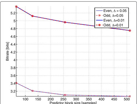
We now quantize as well as entropy code the residual and the LPC coefficients and will therefore be able to obtain bitrates as well as ODG scores. For training the entropy coders, we use a collection of different music genres con-stituting about 5 min of audio sampled at 48 kHz. The test data is the same as above and is not part of the train-ing data. The resulttrain-ing bitrates (expressed in bits/sample) for the even and odd descriptions are shown in Figure 12. The corresponding ODGs are shown in Figures 13 and 14 for = 0.05 and = 0.01, respectively. Interest-ingly, the bitrate (per sample) as well as the ODG are improving as a function of the block size upon which the predictor is applied. Intuitively, one would think that a fixed-order predictor would be better on shorter segments of the signal. We ascribe this phenomenon to the fact that the performance of the current predictor depends upon

Table 6 Average ODG at 1% packet losses

Block size 64 128 256 512 1,024 2,048

=0.01

plpc=5 -0.99 -0.94 -0.40 -0.46 -0.43 -0.37

plpc=10 -0.42 -0.43 -0.32 -0.35 -0.36 -0.34

=0.05

plpc=5 -1.87 -1.81 -1.73 -1.32 -1.17 -1.09

plpc=10 -1.50 -1.39 -1.23 -1.28 -1.25 -1.16

Table 7 Average ODG at 10% packet losses

Block size 64 128 256 512 1,024 2,048

=0.01

plpc=5 -2.77 -2.16 -1.20 -0.87 -0.60 -0.60

plpc=10 -2.61 -1.88 -1.45 -1.08 -0.72 -0.67

=0.05

plpc=5 -3.31 -3.00 -2.49 -2.44 -2.19 -2.16

plpc=10 -3.25 -2.97 -2.93 -2.85 -2.61 -2.35

the predictor applied in the previous block due to the fil-ter’s memory (i.e., we reuse the state of the past predictor). Thus, for short blocks, a substantial part of the prediction of the block is influenced by the history of the previous predictor. This phenomenon is particularly pronounced in the case of large packet-loss rates, where the ODG is sig-nificantly improved by going from block sizes of, e.g., 64 to 512 samples.

4.3 Comparison to existing works

It is interesting to compare the performance of the pro-posed coder to the noise-shaped MD coder presented in [8]. The coder in [8] is based upon the principle of moving horizon (MH) estimation, which is also known as model predictive control when applied in closed-loop control [32]. The scheme in [8] does not use source prediction, and it is therefore expected to perform worse than the pro-posed coder, which combines noise shaping with source prediction. It is also important to note that the scheme in [8] is of ultra low delay, which means that it can operate on small block sizes. Indeed, in the present simulation, we use a block size of one sample. Instead of oversampling, the MDs in [8] are based on the index assignment construc-tion derived in [33]. The simulaconstruc-tion results are presented

100 150 200 250 300 350 400 450 500

3.2 3.4 3.6 3.8 4 4.2 4.4 4.6 4.8 5 5.2

Predictor block size [samples]

Bitrate [bits]

Even, = 0.05 Odd, =0.05 Even, =0.01 Odd, =0.01

Figure 13ODG as a function of predictor block size for₌0.05 and forλ₌1/100.

in Figure 15. The jazz music signal has been used, and two packet loss scenarios have been simulated, a high loss (10% packet losses) and a low loss (1% packet losses) sce-nario. For the proposed coder, we varyin the interval 0.01 to 0.05 in steps of 0.01. The total bitrate consists of the rates required for coding the LSF coefficients as well as the prediction residual. It can be see in the figure that the proposed coder is able to efficiently exploit its prediction loops and thereby reduce the bitrate over what is possible with the MH design. In these simulations, the proposed coder uses a block size of 64 samples for the prediction. Further improvement is possible by increasing the block size.

5 Conclusions

We presented a practical design of a low-delay MD audio coder, which is able to provide a certain degree of robustness towards packet losses. The proposed coder

Figure 14ODG as a function of predictor block size for=0.01 and forλ=1/100.

Figure 15ODG as a function of bitrates for the proposed DSQ scheme and the MD scheme of [8].

combined oversampling and noise shaping with source prediction. The oversampling process creates two source descriptions in order to counteract possible packet losses on the network. The prediction loop removes source redundancy and thereby reduces the coding rate, whereas the noise-shaping process controls the dis-tortion due to receiving subsets of the descriptions. The quantized prediction residual was entropy coded using a static and memoryless Huffman coder. In prac-tical simulations on real audio, it was shown that it is enough to use LPC filters of order 10 (estimated from blocks of 64 samples), noise-shaping filters of order 10, resampling filters of order 200, and bitrates of approximately 4 bits per sample (per description) in order to achieve good quality (ODG better than -1) music in the presence of 1% packet losses.

Endnotes

a_{In layered source coding, the source is usually split}

into a base layer and at least one refinement layer. While the base layer can be used by itself, the refinement layers are usually no good without the base layer.

b_{For reproducibility, the complete source code for the}

proposed coding scheme is electronically available at http://kom.aau.dk/~jo.

c_{The audio signal ‘Abba’ is a 10-s clip of the song ‘Head}

Over Heals’ by Abba - sampled at 44.1 kHz.

d_{In order to correctly estimate the error, we need to}

correct the phase shift of the odd samples. This is done by once more filtering the odd samples with the same filter. Of course, for subjective listening tests, we do not need to correct the phase.

e_{The effect of receiving different numbers of}

Competing interests

The authors declare that they have no competing interests.

Authors’ information

The work of J. Leegaard was performed while he was affiliated with the Department of Electronic System, Aalborg University. He is now with the Department of Architecture, Design and Media Technology, Aalborg University.

Author details

1_{Department of Electronic Systems, Aalborg University, Niels Jernes Vej 12,}

Aalborg 9220, Denmark.2_{Department of Electrical Engineering-Systems, Tel}

Aviv University, Ramat Aviv, Tel Aviv 69978, Israel.

Received: 17 December 2013 Accepted: 31 March 2014 Published: 22 April 2014

References

1. C Chafe, M Gurevich, G Leslie, S Tyan, Effect of time delay on ensemble accuracy, inProc Intl. Soc. Musical Acoustics; Nara, (2004)

2. International Standard ISO/IEC 11172-3 (MPEG), Information technology — coding of moving pictures and associated audio for digital storage media up to about 1.5 mbit/s. Part 3: Audio (1993)

3. International Standard ISO/IEC 13818-7, Information technology – generic coding of moving pictures and associated audio information – Part 7: Advanced Audio Coding (AAC) (2006)

4. International Standard ISO/IEC 14496-3:2005/Amd 2, MPEG 4 Audio profile - high efficiency advanced audio coding (2006)

5. M Bosi, RE Goldberg,Introduction to Digital Audio Coding and Standards (Kluwer Academic Publishers, 2003)

6. GDT Schuller, B Yu, D Huang, B Edler, Perceptual audio coding using adaptive pre-and post-filters and lossless compression. IEEE Trans. Speech Audio Process.10(6), 379–390 (2002)

7. G Simkus, M Holters, U Zoler, Ultra-low delay lossy audio coding using DPCM and block companded quantization, inAustralian Communications

Theory Workshop (AusCTW)(2013), pp. 43–46

8. J Østergaard, DE Quevedo, J Jensen, Real-time perceptual

moving-horizon multiple-description audio coding. IEEE Trans. Signal Process.59(9), 4286–4299 (2011)

9. VK Goyal, Multiple description coding: compression meets the network. IEEE Signal Process. Mag.18(5), 74–93 (2001)

10. J Østergaard, OA Niamut, J Jensen, R Heusdens, Perceptual audio coding using n-channel lattice vector quantization, inIEEE Int. Conf. Acoustics,

Speech, and Signal Processing, vol. 5; Toulouse(2006), pp. 197–200

11. R Arean, J Kovacevic, VK Goyal, Multiple description perceptual audio coding with correlating transform. IEEE Trans. Speech Audio Process. 8, 140–145 (2000)

12. G Schuller, J Kovacevic, F Masson, VK Goyal, Robust low-delay audio coding using multiple descriptions. IEEE Trans. Speech Audio Process. 13, 1014–1024 (2005)

13. J Østergaard, R Zamir, Multiple description coding by dithered delta-sigma quantization. IEEE Trans. Inform. Theor.55(10), 4661–4675 (2009)

14. Y Kochman, J Østergaard, R Zamir, Noise-shaped predictive coding for multiple descriptions of a colored gaussian source, inIEEE Data

Compression Conference (DCC)(Snowbird Utah, 2008), pp. 362–371

15. J Østergaard, Y Kochman, R Zamir, Colored gaussian multiple descriptions: spectral-domain characterization and time-domain design. Submitted to IEEE Transactions on Information Theory (2010). Electronically available on arXiv.org: http://arxiv.org/abs/1006.2002 16. RE Crochiere, LR Rabiner, Interpolation and decimation of digital signals

— a tutorial review. Proc. IEEE69(3), 300–331 (1981)

17. JO Smith, P Gossett, A flexible sampling-rate conversion method, in Proceedings of the International Conference on Acoustics, Speech, and Signal

Processing; San Diego(1984)

18. AJ Russel, PE Beckmann, Efficient arbitrary sampling rate conversion with recursive calculation of coefficients. IEEE Trans. Signal Process. 50, 854–865 (2002)

19. R Zamir, Y Kochman, U Erez, Achieving the gaussian rate-distortion function by prediction. IEEE Trans. Inform. Theor.54(7), 3354–3364 (2008)

20. M Palgy, J Østergaard, R Zamir, Multiple description image/video compression using oversampling and noise shaping in the DCT domain, inIEEE 26th Convention of Electrical and Electronics Engineers in Israel (Eilat Israel, 2010)

21. SK Tewksbury, RW Hallock, Oversampled, linear predictive and noise-shaping coders of ordern>1. IEEE Trans. Circ. Syst.CAS-25(7), 436–447 (1978)

22. TW Parks, JH McClellan, Chebyshev approximation for nonrecursive digital filters with linear phase. IEEE Trans. Circ. Theor.ct-19, 189–194 (1972) 23. D O’Shaughnessy, Linear predictive coding. IEEE Potentials7(1), 29–32

(1988)

24. J Klejsa, WB Kleijn, Rate distribution between model and signal for multiple descriptions, inIEEE International Conference on Acoustics, Speech

and Signal Processing; Taipei, (2009), pp. 2489–2492

25. RM Gray, DL Neuhoff, Quantization. IEEE Trans. Inform. Theor. 44(6), 2325–2383 (1998)

26. DA Huffman, A method for the construction of minimum-redundancy codes. Proc. IRE40(9), 1098–1101 (1952)

27. WB Kleijn, KK Paliwal (eds.),Speech Coding and Synthesis, 1st edn. (Elsevier, 1995)

28. F Itakura, Line spectrum representation of linear predictor coefficients of speech signals. J. Acoust. Soc. Amer.57(1975)

29. FK Soong, B Juang, Optimal quantization of LSP parameters. IEEE Trans. Speech Audio Process.1, 15–24 (1993)

30. ITU-R Recommendation BS.1387, Perceptual Evaluation of Audio Quality (PEAQ) (1998)

31. P Kabal, An examination and interpretation of itu-r bs.1387: perceptual evaluation of audio quality. Technical report, McGill University. Version 2 (2003)

32. GC Goodwin, MM Seron, JAD Dona,Constrained Control and Estimation:

An Optimisation Approach. (Springer, 2005)

33. J Østergaard, J Jensen, R Heusdens, n-channel entropy-constrained multiple-description lattice vector quantization. IEEE Trans. Inform. Theor. 52(5), 1956–1973 (2006)

34. A Mashiach, J Østergaard, R Zamir, Sampling versus random binning for multiple descriptions of a bandlimited source, inIEEE Information Theory Workshop; Seville, (2013)

doi:10.1186/1687-4722-2014-16

Cite this article as:Leegaardet al.:Practical design of delta-sigma multiple description audio coding. EURASIP Journal on Audio, Speech, and Music Processing20142014:16.

Submit your manuscript to a

journal and benefi t from:

7Convenient online submission

7Rigorous peer review

7Immediate publication on acceptance

7Open access: articles freely available online

7High visibility within the fi eld

7Retaining the copyright to your article