Automatic focus algorithms for TDI X-Ray image reconstruction

(1)

Adv. Radio Sci., 10, 145–151, 2012 www.adv-radio-sci.net/10/145/2012/ doi:10.5194/ars-10-145-2012

Advances in

Radio Science

Automatic focus algorithms for TDI X-Ray image reconstruction

J. D¨orr, M. Rosenbaum, W. Sauer-Greff, and R. Urbansky

TU Kaiserslautern, Institute of Communications Engineering, 67653 Kaiserslautern, Germany Correspondence to: M. Rosenbaum ([email protected])

Abstract. In food industry, most products are checked by X-rays for contaminations. These X-ray machines contin-uously scan the product passing through. To minimize the required X-ray power, a Time, Delay and Integration (TDI) CCD-sensor is used to capture the image. While the prod-uct moves across the sensor area, the X-ray angle changes during the pass. As a countermeasure, adjusting the sensor shift speed on a single focal plane of the product can be se-lected. However, the changing angle result in a blurred image in dependance to the thickness of the product. This so-called “laminographic effect” can be compensated individually for one plane by inverse filtering. As the plane of contamination is unknown, the blurred image will be inversely filtered for different planes, but only one of these images shows the cor-rectly focussed object. If the correct image can be found, the plane containing the contamination is identified. In this con-tribution we demonstrate how the correctly focussed images can be found by analyzing the images of all planes. Different characteristics for correctly and incorrectly focussed planes like sharpness, number of objects and edges are investigated by using image processing algorithms.

1 Introduction

For quality assurance in food industry more and more X-ray-scanners are used instead of simple metal detectors, because they are also able to detect non-metallic contaminations, to check filling levels or to check that a product is sealed prop-erly. For such scanning applications continuous processing is desirable, because it fits in most production processes with-out the need of further adaptations. To minimize the required X-ray power, a Time, Delay and Integration (TDI) (Wong et al., 1992) CCD sensor can be used to capture images while the objects are moving across the sensor area. One way to ob-tain depth information is the use of laminographic techniques (Gondrom and Schr¨opfer, 1999; Rooks and Sack, 1995) in

Manuscript prepared for Adv. Radio Sci.

with version 4.2 of the LA_{TEX class copernicus.cls.} Date: 27 July 2012

Automatic Focus Algorithms for TDI X-Ray Image Reconstruction

J. D¨orr, M. Rosenbaum, W. Sauer-Greff, and R. Urbansky

TU Kaiserslautern, Institute of Communications Engineering, 67653 Kaiserslautern, Germany

Abstract. In food industry, most products are checked by X-rays for contaminations. These X-ray machines contin-uously scan the product passing through. To minimize the required X-ray power, a Time, Delay and Integration (TDI) CCD-sensor is used to capture the image. While the prod-5

uct moves across the sensor area, the X-ray angle changes during the pass. As a countermeasure, adjusting the sensor shift speed on a single focal plane of the product can be se-lected. However, the changing angle result in a blurred image in dependance to the thickness of the product. This so-called 10

,,laminographic effect” can be compensated individually for one plane by inverse filtering. As the plane of contamination is unknown, the blurred image will be inversely filtered for different planes, but only one of these images shows the cor-rectly focussed object. If the correct image can be found, the 15

plane containing the contamination is identified. In this con-tribution we demonstrate how the correctly focussed images can be found by analyzing the images of all planes. Different characteristics for correctly and incorrectly focussed planes like sharpness, number of objects and edges are investigated 20

by using image processing algorithms.

1 Introduction

For quality assurance in food industry more and more X-ray-scanners are used instead of simple metal detectors, because 25

they are also able to detect non-metallic contaminations, to check filling levels or to check that a product is sealed prop-erly. For such scanning applications continuous processing is desirable, because it fits in most production processes with-out the need of further adaptations. To minimize the required 30

X-ray power, a Time, Delay and Integration (TDI) (Wong et al. (1992)) CCD sensor can be used to capture images while Correspondence to: Mark Rosenbaum

([email protected])

a)

transport belt product

CCD-sensor with lines α1

X-ray source

t2

t1 t3 α3 α2

b)

transport belt product

CCD-Sensor with lines

X-ray source

t2

t1 t3

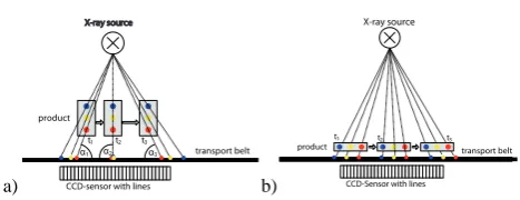
Fig. 1. The laminographic effect: result of changing angle on (a)

high objects (b) no impact on flat objects

the objects are moving across the sensor area. One way to ob-tain depth information is the use of laminographic techniques (Gondrom, Schr¨opfer (1999), Rooks, Sack (1995)) in con-35

junction with the Radon Transform (Popularikas (1996)). This requires a complex mechanical setup not suitable for continuous scanning or requires two or more X-ray sources and detectors. This approach is not only expensive in terms of investment, in addition the second X-ray tube also needs 40

power, cooling and better shielding against X-rays leaving the machine.

An alternative way is the use of a single sensor followed by inverse filtering. However, this technique causes the problem that the angle of the X-rays changes during the transport, as 45

shown in figure 1.

This effect can be modeled as a convolution of the real im-agea(x,y)with the point spread function (PSF) of the imag-ing systemh(x,y), yielding an images(x,y).

s(x,y) =a(x,y)∗h(x,y) (1)

50

In general, this PSF is two-dimensional, but in our case only the contribution in direction of the belt movement is significant, which can be modeled as a one-dimensional im-pulse response. This impulse response is height variant, which means it is only valid for a given height of the object 55

Fig. 1. The laminographic effect: result of changing angle on (a)

high objects (b) no impact on flat objects

conjunction with the Radon Transform (Popularikas, 1996). This requires a complex mechanical setup not suitable for continuous scanning or requires two or more X-ray sources and detectors. This approach is not only expensive in terms of investment, in addition the second X-ray tube also needs power, cooling and better shielding against X-rays leaving the machine.

An alternative way is the use of a single sensor followed by inverse filtering. However, this technique causes the problem that the angle of the X-rays changes during the transport, as shown in Fig. 1.

This effect can be modeled as a convolution of the real imagea(x,y) with the point spread function (PSF) of the imaging systemh(x,y), yielding an images(x,y).

s(x,y)=a(x,y)∗h(x,y) (1) In general, this PSF is two-dimensional, but in our case only the contribution in direction of the belt movement is sig-nificant, which can be modeled as a one-dimensional im-pulse response. This impulse response is height variant, which means it is only valid for a given height of the object above the sensor plane. Further information can be found in (Rosenbaum et al., 2011).

Images of thin objects can be deblurred by inverse filtering during post processing using a Wiener filter approach. This

(2)

146 J. D¨orr et al.: Automatic focus algorithms for TDI X-Ray image reconstruction

deblurring process performs well for thin objects, if the PSF is known. The PSF can be estimated for one specific plane or layer. By resizing this PSF one can obtain PSFs of other layers. However, it is unknown which layer contains the con-tamination. So the idea is to deblur the image with respect to the PSFs of different layers and to search for a correctly focussed image a posteriori. If no correctly focussed image can be identified, the object is not flat. If a correct image is found, the object is flat and the height of the object over the transport belt is known.

Humans are well able to decide for correctly focussed im-ages. However, for practical industrial usage the decision has to be made by computer algorithms. Unfortunately, stan-dard autofocus algorithms (Subbarao et al., 1993) can not be applied because of potential artifacts from inverse filtering. In this article a solution for these problems is proposed and demonstrated by simulation results.

The remainder of this paper is organized as follows: Af-ter an overview on inverse filAf-tering which is visualized by resulting images from our simulation setup, three different autofocus algorithms are discussed. A combination of these algorithms is proposed and demonstrated by simulation re-sults. Finally, conclusions are drawn.

2 Simulation setup

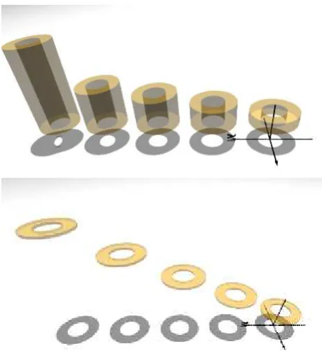
To demonstrate and test the proposed algorithms, the ray tracing software POV-Ray (see www.povray.org) was used to build test images, where a visual light source models the X-ray tube. Figure 2 shows the model. Different washers and cylinders with different thicknesses in different layers were simulated. To model the conveyor belt, the light source is moved and the changing shadows are captured. Finally, the images of different light positions are merged to one image by calculating the mean value. This simulates the lamino-graphic effect resulting from the use of an TDI X-ray system. The results of the mean value calculations are inversely filtered for a specific number of layers (here 160). Finally we use these 160 inversely filtered layer-images for every washer to test the algorithms.

3 Inverse filtering

Blurring caused by the laminographic effect can be effec-tively addressed by inverse filtering since it can be regarded as a convolution of the real image with the point-spread-function of the imaging system additionally corrupted with noisen.

s(x,y)=a(x,y)∗h(x,y)+n (2) The inverse filtering takes advantage of the frequency do-main. A pure inversion of the transfer functionH (fx,fy)

requires to take the reciprocal of it yieldingHw(fx,fy)=

2 J. D¨orr et al.: Automatic Focus Algorithms for TDI X-Ray Image Reconstruction

above the sensor plane. Further information can be found in (Rosenbaum et al. (2011)).

Images of thin objects can be deblurred by inverse filtering during post processing using a Wiener filter approach. This deblurring process performs well for thin objects, if the PSF 60

is known. The PSF can be estimated for one specific plane or layer. By resizing this PSF one can obtain PSFs of other layers. However, it is unknown which layer contains the con-tamination. So the idea is to deblur the image with respect to the PSFs of different layers and to search for a correctly 65

focussed image a posteriori. If no correctly focussed image can be identified, the object is not flat. If a correct image is found, the object is flat and the height of the object over the transport belt is known.

Humans are well able to decide for correctly focussed im-70

ages. However, for practical industrial usage the decision has to be made by computer algorithms. Unfortunately, standard autofocus algorithms (Subbarao et al. (1993)) can not be applied because of potential artifacts from inverse filtering. In this article a solution for these problems is proposed and 75

demonstrated by simulation results.

The remainder of this paper is organized as follows: Af-ter an overview on inverse filAf-tering which is visualized by resulting images from our simulation setup, three different autofocus algorithms are discussed. A combination of these 80

algorithms is proposed and demonstrated by simulation re-sults. Finally, conclusions are drawn.

2 Simulation Setup

To demonstrate and test the proposed algorithms, the ray tracing software POV-Ray (see www.povray.org) was used 85

to build test images, where a visual light source models the X-ray tube. Figure 2 shows the model. Different washers and cylinders with different thicknesses in different layers were simulated. To model the conveyor belt, the light source is moved and the changing shadows are captured. Finally, the 90

images of different light positions are merged to one image by calculating the mean value. This simulates the lamino-graphic effect resulting from the use of an TDI X-ray system. The results of the mean value calculations are inversely filtered for a specific number of layers (here 160). Finally 95

we use these 160 inversely filtered layer-images for every washer to test the algorithms.

3 Inverse Filtering

Blurring caused by the laminographic effect can be effec-tively addressed by inverse filtering since it can be regarded 100

as a convolution of the real image with the point-spread-function of the imaging system additionally corrupted with noisen.

s(x,y) =a(x,y)∗h(x,y) +n (2)

Fig. 2. Ray tracing model to test algorithms

Fig. 3. Block diagram of the whole imaging process

The inverse filtering takes advantage of the frequency do-105

main. A pure inversion of the transfer functionH(fx,fy)

requires to take the reciprocal of it yieldingHw(fx,fy) =

H−1_(f

x,fy), which poses problems because of spectral

ze-ros and ampluification of noise contained in the X-ray im-age. A well-known solution to this problem is Wiener filter-110

ing (Madissettti and Williams (1998)). Equation 3 shows the parametric form of the Wiener filter.Kaccounts for noise in-fluence, which is ideally chosen as the reciprocal of the input signal-to-noise-ratio.

Hw(fx,fy) =

H∗_(f

x,fy)

|H(fx,fy)|2+K

(3) 115

Figure 3 summarizes the imaging and reconstruction process, which produces an estimateAˆof the unknown original image A

In the reconstruction process, an impulse response is only valid for a single focal plane. The characteristics of the imag-120

ing process allow to calculate an impulse response for every Fig. 2. Ray tracing model to test algorithms.

2 J. D¨orr et al.: Automatic Focus Algorithms for TDI X-Ray Image Reconstruction above the sensor plane. Further information can be found in

(Rosenbaum et al. (2011)).

Images of thin objects can be deblurred by inverse filtering during post processing using a Wiener filter approach. This deblurring process performs well for thin objects, if the PSF 60

is known. The PSF can be estimated for one specific plane or layer. By resizing this PSF one can obtain PSFs of other layers. However, it is unknown which layer contains the con-tamination. So the idea is to deblur the image with respect to the PSFs of different layers and to search for a correctly 65

focussed image a posteriori. If no correctly focussed image can be identified, the object is not flat. If a correct image is found, the object is flat and the height of the object over the transport belt is known.

Humans are well able to decide for correctly focussed im-70

ages. However, for practical industrial usage the decision has to be made by computer algorithms. Unfortunately, standard autofocus algorithms (Subbarao et al. (1993)) can not be applied because of potential artifacts from inverse filtering. In this article a solution for these problems is proposed and 75

demonstrated by simulation results.

The remainder of this paper is organized as follows: Af-ter an overview on inverse filAf-tering which is visualized by resulting images from our simulation setup, three different autofocus algorithms are discussed. A combination of these 80

algorithms is proposed and demonstrated by simulation re-sults. Finally, conclusions are drawn.

2 Simulation Setup

To demonstrate and test the proposed algorithms, the ray tracing software POV-Ray (see www.povray.org) was used 85

to build test images, where a visual light source models the X-ray tube. Figure 2 shows the model. Different washers and cylinders with different thicknesses in different layers were simulated. To model the conveyor belt, the light source is moved and the changing shadows are captured. Finally, the 90

images of different light positions are merged to one image by calculating the mean value. This simulates the lamino-graphic effect resulting from the use of an TDI X-ray system. The results of the mean value calculations are inversely filtered for a specific number of layers (here 160). Finally 95

we use these 160 inversely filtered layer-images for every washer to test the algorithms.

3 Inverse Filtering

Blurring caused by the laminographic effect can be effec-tively addressed by inverse filtering since it can be regarded 100

as a convolution of the real image with the point-spread-function of the imaging system additionally corrupted with noisen.

s(x,y) =a(x,y)∗h(x,y) +n (2)

Fig. 2. Ray tracing model to test algorithms

Fig. 3. Block diagram of the whole imaging process

The inverse filtering takes advantage of the frequency do-105

main. A pure inversion of the transfer functionH(fx,fy)

requires to take the reciprocal of it yieldingHw(fx,fy) =

H−1_(f

x,fy), which poses problems because of spectral

ze-ros and ampluification of noise contained in the X-ray im-age. A well-known solution to this problem is Wiener filter-110

ing (Madissettti and Williams (1998)). Equation 3 shows the parametric form of the Wiener filter.Kaccounts for noise in-fluence, which is ideally chosen as the reciprocal of the input signal-to-noise-ratio.

Hw(fx,fy) =

H∗_(f

x,fy)

|H(fx,fy)|2+K

(3) 115

Figure 3 summarizes the imaging and reconstruction process, which produces an estimateAˆof the unknown original image A

In the reconstruction process, an impulse response is only valid for a single focal plane. The characteristics of the imag-120

ing process allow to calculate an impulse response for every Fig. 3. Block diagram of the whole imaging process.

H−1(fx,fy), which poses problems because of spectral

ze-ros and amplification of noise contained in the X-ray image. A well-known solution to this problem is Wiener filtering (Madissettti and Williams, 1998). Equation (3) shows the parametric form of the Wiener filter. K accounts for noise influence, which is ideally chosen as the reciprocal of the in-put signal-to-noise-ratio.

Hw(fx,fy)=

H∗(fx,fy)

|H (fx,fy)|2+K

(3) Figure 3 summarizes the imaging and reconstruction pro-cess, which produces an estimateAˆof the unknown original imageA.

In the reconstruction process, an impulse response is only valid for a single focal plane. The characteristics of the imag-ing process allow to calculate an impulse response for every focal plane out of one known impulse response by using al-gorithms also known in image processing as bilinear or bicu-bic scaling (details can be found in Keys, 1981).

(3)

J. D¨orr et al.: Automatic focus algorithms for TDI X-Ray image reconstruction 147

J. D¨orr et al.: Automatic Focus Algorithms for TDI X-Ray Image Reconstruction

3

Fig. 4. Blurred image with compressed PSF

Fig. 5. Inversely filtered with lightly spread PSF

focal plane out of one known impulse response by using

al-gorithms also known in image processing as bilinear or

bicu-bic scaling (details can be found in (Keys (1981))).

To estimate the height of an object above the belt, images

125

have to be reconstructed with scaled PSFs. In our case, 160

images corresponding to 160 focal planes with a distance of

0,5mm were calculated, yielding a range of 8 cm. As

de-scribed in section 2, we used simulated X-ray scenarios of

a thin metallic washer, diameter 2cm. Some examples of

130

these images are shown in figures 4 - 7. The characteristics

of these images and especially the differences between the

correctly and incorrectly focussed images will be useful for

understanding suitable algorithms.

If the inverse filtering PSF is too compressed, it nearly

cor-135

responds to a dirac-impulse and therefore the result of the

convolution with this PSF resembles the original blurred

im-age after the scanning process (figure 4). The result is a very

blurry image, but it shows only one object and not separated

parts of the washer. Figure 5 depicts the result of an inverse

140

convolution with a wider spread PSF. If the PSF is spread

farther, artifacts with sharp edges and many separated areas

Fig. 6. Many separated objects and edges are the result of inverse filtering with widely spread PSF

a) b)

Fig. 7. Results of inversion with correctly scaled PSF a) washer on a low layer, b) washer on a high layer

Figure 7 depicts an example for images filtered with the

correctly scaled PSF and which should be chosen as correctly

145

focussed. They are characterized by sharp edges, only one

object and not many changes of intensity values.

4 Algorithms

In general, the contaminants cannot be specified and the

product may also vary.

This means, the general

proper-150

ties which are different between correctly and incorrectly

fo-cussed images need to be used to detect the focal plane.

In this contribution we propose to use the set of

follow-ing features: (1) peaks of image autocorrelation function, (2)

number of objects and (3) pixels outside objects.

155

4.1 Autocorrelation

Incorrectly focussed images with a too wide PSF suffer from

periodic artifacts, which need to be detected. The idea is to

Fig. 4. Blurred image with compressed PSF.

J. D¨orr et al.: Automatic Focus Algorithms for TDI X-Ray Image Reconstruction 3

focal plane out of one known impulse response by using al-gorithms also known in image processing as bilinear or bicu-bic scaling (details can be found in (Keys (1981))).

To estimate the height of an object above the belt, images 125

have to be reconstructed with scaled PSFs. In our case, 160 images corresponding to 160 focal planes with a distance of 0,5mm were calculated, yielding a range of 8 cm. As de-scribed in section 2, we used simulated X-ray scenarios of a thin metallic washer, diameter 2cm. Some examples of 130

these images are shown in figures 4 - 7. The characteristics of these images and especially the differences between the correctly and incorrectly focussed images will be useful for understanding suitable algorithms.

If the inverse filtering PSF is too compressed, it nearly cor-135

responds to a dirac-impulse and therefore the result of the convolution with this PSF resembles the original blurred im-age after the scanning process (figure 4). The result is a very blurry image, but it shows only one object and not separated parts of the washer. Figure 5 depicts the result of an inverse 140

convolution with a wider spread PSF. If the PSF is spread farther, artifacts with sharp edges and many separated areas are the result as shown in figure 6.

Fig. 6. Many separated objects and edges are the result of inverse

filtering with widely spread PSF

a) b)

Fig. 7. Results of inversion with correctly scaled PSF a) washer on

a low layer, b) washer on a high layer

Figure 7 depicts an example for images filtered with the correctly scaled PSF and which should be chosen as correctly 145

focussed. They are characterized by sharp edges, only one object and not many changes of intensity values.

4 Algorithms

In general, the contaminants cannot be specified and the product may also vary. This means, the general proper-150

ties which are different between correctly and incorrectly fo-cussed images need to be used to detect the focal plane.

In this contribution we propose to use the set of follow-ing features: (1) peaks of image autocorrelation function, (2) number of objects and (3) pixels outside objects.

155

4.1 Autocorrelation

Incorrectly focussed images with a too wide PSF suffer from periodic artifacts, which need to be detected. The idea is to measure these changes by autocorrelation. The more peri-Fig. 5. Inversely filtered with lightly spread PSF.

To estimate the height of an object above the belt, im-ages have to be reconstructed with scaled PSFs. In our case, 160 images corresponding to 160 focal planes with a dis-tance of 0.5 mm were calculated, yielding a range of 8 cm. As described in Sect. 2, we used simulated X-ray scenarios of a thin metallic washer, diameter 2 cm. Some examples of these images are shown in Figs. 4–7. The characteristics of these images and especially the differences between the correctly and incorrectly focussed images will be useful for understanding suitable algorithms.

If the inverse filtering PSF is too compressed, it nearly cor-responds to a dirac-impulse and therefore the result of the convolution with this PSF resembles the original blurred im-age after the scanning process (Fig. 4).

The result is a very blurry image, but it shows only one object and not separated parts of the washer. Figure 5 depicts the result of an inverse convolution with a wider spread PSF. If the PSF is spread farther, artifacts with sharp edges and many separated areas are the result as shown in Fig. 6.

Figure 7 depicts an example for images filtered with the correctly scaled PSF and which should be chosen as correctly focussed. They are characterized by sharp edges, only one object and not many changes of intensity values.

4 Algorithms

In general, the contaminants cannot be specified and the product may also vary. This means, the general

proper-J. D¨orr et al.: Automatic Focus Algorithms for TDI X-Ray Image Reconstruction 3

a) b)

4 Algorithms

155

Incorrectly focussed images with a too wide PSF suffer from periodic artifacts, which need to be detected. The idea is to measure these changes by autocorrelation. The more peri-Fig. 6. Many separated objects and edges are the result of inverse

filtering with widely spread PSF.

a) b)

4 Algorithms

155

Incorrectly focussed images with a too wide PSF suffer from periodic artifacts, which need to be detected. The idea is to measure these changes by autocorrelation. The more peri-Fig. 7. Results of inversion with correctly scaled PSF (a) washer on

a low layer, (b) washer on a high layer.

Incorrectly focussed images with a too wide PSF suffer from periodic artifacts, which need to be detected. The idea is to measure these changes by autocorrelation. The more peri-odic artifacts appear in an image, the more peaks occur in the result of the image autocorrelation function.

The autocorrelation function is calculated for every image line. Figure 8 shows the resulting matrix after normalization. After the summation of all lines the result is a ,,correlation line”. To deal with varying image intensities, the maximum of the autocorrelation function is normalized to 1. Figure 9 shows an example for an autocorrelation function of a cor-rectly focussed image and Fig. 10 for an incorcor-rectly focussed image.

Obviously, the incorrectly focussed image produces more autocorrelation peaks than the correctly focussed. We pro-pose to sum up the number of peaks of the correlation line. These sums for all images over the image height index are shown in Fig. 11. The value near the best image is very low in comparison to incorrectly focussed images. As can be seen, this criterion is suitable expect for low-index (compressed

(4)

1484 J. D¨orr et al.: Automatic focus algorithms for TDI X-Ray image reconstructionJ. D¨orr et al.: Automatic Focus Algorithms for TDI X-Ray Image Reconstruction

Fig. 8. Example of correlation matrix

0 100 200 300 400 500 600 700

0 0.2 0.4 0.6 0.8 1

Fig. 9. Correlation line with one object (correctly focussed)

odic artifacts appear in an image, the more peaks occur in 160

the result of the image autocorrelation function.

The autocorrelation function is calculated for every image line. Figure 8 shows the resulting matrix after normalization. After the summation of all lines the result is a ,,correlation line”. To deal with varying image intensities, the maximum 165

of the autocorrelation function is normalized to 1. Figure 9 shows an example for an autocorrelation function of a cor-rectly focussed image and figure 10 for an incorcor-rectly fo-cussed image.

Obviously, the incorrectly focussed image produces more 170

autocorrelation peaks than the correctly focussed. We pro-pose to sum up the number of peaks of the correlation line. These sums for all images over the image height index are shown in figure 11. The value near the best image is very low in comparison to incorrectly focussed images. As can 175

be seen, this criterion is suitable expect for low-index (com-pressed PSF) images. So, for these images another algorithm has to be employed.

4.2 Object Count

Another difference between a correctly and most of the incor-180

rectly focussed images is the number of separated objects. To count the objects, an area has to be defined and divided into seperate objects. This is done by a binarisation and a follow-ing object segmentation. The binarisation threshold has to be determined adaptively depending on the background bright-185

ness.

0 100 200 300 400 500 600 700

0 0.2 0.4 0.6 0.8 1

Fig. 10. Correlation line with multiple objects (PSF too wide,

in-correctly focussed)

Fig. 11. Sum of maxima over image index, correctly focussed

im-age leads to low values, but there are also imim-ages with lower values.

All connected white pixels are counted as one object. To find out which pixel groups belong together, well known seg-mentation algorithms (Ho (2011)) can be used.

Figure 12 shows two binarized images. Obviously, the 190

incorrectly focussed image contains more objects (white ar-eas) than the correctly focussed image. Figure 13 shows the counted number of objects over the image height index.

Obviously many images have only one object, especially the low index images and the images around the correctly 195

focussed image.

This algorithm is more likely usable for an image pre-selection because it cannot determine the correctly focussed image, but it can detect images which are clearly incorrectly focussed.

200

4.3 Remaining Pixel Analysis

The two previous algorithms work well if the PSF is widely spread. They fail for blurred images, which result from in-verse filtering with a narrow PSF. A possible solution for this problem is to count the pixels which remain outside the ob-205

jects after binarisation. This can be implemented very effi-ciently: The filtered image with white background is bina-rized after applying a noise suppressing Gaussian filter. This binarized image is multiplied with the inverted image. Since the color black corresponds to the value zero all pixels in ob-210

ject areas are suppressed. The number of remaining pixels will be summed up.

Figure 14 demonstrates the process, and figure 15 shows the sums of remaining pixels over the image hight index. As Fig. 8. Example of correlation matrix.

0 100 200 300 400 500 600 700

0 0.2 0.4 0.6 0.8 1

ness.

0 100 200 300 400 500 600 700

0 0.2 0.4 0.6 0.8 1

focussed image.

200

Figure 14 demonstrates the process, and figure 15 shows the sums of remaining pixels over the image hight index. As Fig. 9. Correlation line with one object (correctly focussed).

PSF) images. So, for these images another algorithm has to be employed.

4.2 Object count

Another difference between a correctly and most of the incor-rectly focussed images is the number of separated objects. To count the objects, an area has to be defined and divided into seperate objects. This is done by a binarisation and a follow-ing object segmentation. The binarisation threshold has to be determined adaptively depending on the background bright-ness.

All connected white pixels are counted as one object. To find out which pixel groups belong together, well known seg-mentation algorithms (Ho, 2011) can be used.

Figure 12 shows two binarized images. Obviously, the in-correctly focussed image contains more objects (white areas) than the correctly focussed image.

Figure 13 shows the counted number of objects over the image height index.

Obviously many images have only one object, especially the low index images and the images around the correctly focussed image.

4.3 Remaining pixel analysis

The two previous algorithms work well if the PSF is widely spread. They fail for blurred images, which result from

in-4 J. D¨orr et al.: Automatic Focus Algorithms for TDI X-Ray Image Reconstruction

0 100 200 300 400 500 600 700

0 0.2 0.4 0.6 0.8 1

ness.

0 100 200 300 400 500 600 700

0 0.2 0.4 0.6 0.8 1

focussed image.

200

Figure 14 demonstrates the process, and figure 15 shows the sums of remaining pixels over the image hight index. As Fig. 10. Correlation line with multiple objects (PSF too wide,

in-correctly focussed).

0 100 200 300 400 500 600 700

0 0.2 0.4 0.6 0.8 1

ness.

0 100 200 300 400 500 600 700

0 0.2 0.4 0.6 0.8 1

focussed image.

200

Figure 14 demonstrates the process, and figure 15 shows the sums of remaining pixels over the image hight index. As Fig. 11. Sum of maxima over image index, correctly focussed

verse filtering with a narrow PSF. A possible solution for this problem is to count the pixels which remain outside the ob-jects after binarisation. This can be implemented very effi-ciently: The filtered image with white background is bina-rized after applying a noise suppressing Gaussian filter. This binarized image is multiplied with the inverted image. Since the color black corresponds to the value zero all pixels in ob-ject areas are suppressed. The number of remaining pixels will be summed up.

Figure 14 demonstrates the process, and Fig. 15 shows the sums of remaining pixels over the image hight index. As can be seen the process works well, therefore the correctly focussed image can be found easily by a minimum-search. 4.4 Combination of algorithms

Other test images showed that summing up the pixels out of objects could lead to a few wrong decisions. Therefore, a combination of the presented methods is proposed. The flowchart in Fig. 16 illustrates the concept of a full image detection process.

First, the remaining pixels and the number of objects are calculated. In addition, the number of edges are counted. This acts like counting the objects, but with a preceding edge-finding algorithm.

To identify that an image indicates a plane with a flat ob-ject, the following conditions are proposed: A correctly fo-cussed image has to exhibit only one object, not more than a specific number of edges and a sum of remaining pixels lower than a specific threshold, which depends on the edge length. The thresholds have to be adapted to the specific

(5)

J. D¨orr et al.: Automatic focus algorithms for TDI X-Ray image reconstructionJ. D¨orr et al.: Automatic Focus Algorithms for TDI X-Ray Image Reconstruction 5 149

a) b)

Fig. 12. After binarisation only one object in correctly focussed

image (a) many objects in incorrectly focussed image

Fig. 13. number of objects over image index for a washer on a low

layer

can be seen the process works well, therefore the correctly 215

focussed image can be found easily by a minimum-search.

4.4 Combination of Algorithms

Other test images showed that summing up the pixels out of objects could lead to a few wrong decisions. Therefore, a combination of the presented methods is proposed. The 220

flowchart in figure 16 illustrates the concept of a full image detection process.

First, the remaining pixels and the number of objects are calculated. In addition, the number of edges are counted. This acts like counting the objects, but with a preceding edge-225

finding algorithm.

To identify that an image indicates a plane with a flat ob-ject, the following conditions are proposed: A correctly fo-cussed image has to exhibit only one object, not more than a specific number of edges and a sum of remaining pixels 230

lower than a specific threshold, which depends on the edge length. The thresholds have to be adapted to the specific sys-tem. If no image satisfying the conditions can be identified, it is assumed that there is no distinguishable flat object.

To save computing time, the number of edges and the au-235

tocorrelations are calculated for images with one object only. The results of remaining pixels and of autocorrelations are combined to deliver a final result. In our example, the algo-rithm detects three images, which satisfy the conditions and the correct image (index 35 in this example) has been found. 240

a1) b1)

a2) b2)

a3) b3)

Fig. 14. After binarisation (a2, b2) and multiplication with original

(a1,b1) there are many pixels remaining in the result of the blurred image (a1) and only a few pixels in the result of the sharp image (b3)

a)

b)

Fig. 15. Sum of non-black pixels out-of objects a) washer on a low

layer, b) washer on a higher layer

5 Results

Figure 17 shows the results of the steps of the combined al-gorithm for one of the washers. The parameters of the algo-Fig. 12. After binarisation only one object in correctly focussed

image (a) many objects in incorrectly focussed image.

a) b)

layer

finding algorithm.

a1) b1)

a2) b2)

a3) b3)

a)

b)

5 Results

Figure 17 shows the results of the steps of the combined al-gorithm for one of the washers. The parameters of the algo-Fig. 13. Number of objects over image index for a washer on a low

layer.

system. If no image satisfying the conditions can be identi-fied, it is assumed that there is no distinguishable flat object. To save computing time, the number of edges and the au-tocorrelations are calculated for images with one object only. The results of remaining pixels and of autocorrelations are combined to deliver a final result. In our example, the algo-rithm detects three images, which satisfy the conditions and the correct image (index 35 in this example) has been found.

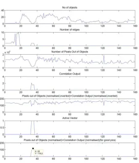
5 Results

Figure 17 shows the results of the steps of the combined al-gorithm for one of the washers. The parameters of the algo-rithms, like threshold values or Gaussian filter values were set up in such a way that they operate successfully for all test images. Objects with a height below 2 centimeters are con-sidered flat, yielding a distinguished sharp plane. For objects higher than that, which are considered non-flat, no erroneous images satisfying the conditions have been found.

6 Conclusions

It has been demonstrated that the proposed technique is able to identify distinguishable flat objects in a set of images re-sulting from inverse filtering of a laminographic image for different focal planes. The algorithm is based on combining methods from autocorrelation techniques, object counts and pixels-outside-objects analysis.

Together with the idea of height variant inverse filtering this paves the way to extracting 3-D-Information out of 2-D scanned objects by using the laminographic effect of

TDI-X-J. D¨orr et al.: Automatic Focus Algorithms for TDI X-Ray Image Reconstruction 5

a) b)

layer

finding algorithm.

a1) b1)

a2) b2)

a3) b3)

a)

b)

5 Results

Figure 17 shows the results of the steps of the combined al-gorithm for one of the washers. The parameters of the algo-Fig. 14. After binarisation (a2, b2) and multiplication with

orig-inal (a1,b1) there are many pixels remaining in the result of the blurred image (a1) and only a few pixels in the result of the sharp image (b3).

a) b)

layer

finding algorithm.

a1) b1)

a2) b2)

a3) b3)

a)

b)

5 Results

Figure 17 shows the results of the steps of the combined al-gorithm for one of the washers. The parameters of the algo-Fig. 15. Sum of non-black pixels out-of objects (a) washer on a low

layer, (b) washer on a higher layer.

ray systems. The concept works well in our simulation setup, the next step will be to verify these results for a real system.

(6)

150 J. D¨orr et al.: Automatic focus algorithms for TDI X-Ray image reconstruction

remaining pixels

store sum of pixel outside objects in vector

for each image

object segmentation number of objects in

image

edge segmenatation

number of edges

no correct image available select images with only

one object

write 1 in vector

calculate edge length

write 0 in vector

find best image

index of correct image

vector

no yes

sum of remaining pixel lower than threshold (5 times the edge length) number of edges lower than threshold

autocorrelation

condition only zeros

in vector zeros and ones

in vector

Fig. 16. Structure of combined process

rithms, like threshold values or Gaussian filter values were set up in such a way that they operate successfully for all test 245

images. Objects with a height below 2 centimeters are con-sidered flat, yielding a distinguished sharp plane. For objects higher than that, which are considered non-flat, no erroneous images satisfying the conditions have been found.

6 Conclusions

250

It has been demonstrated that the proposed technique is able to identify distinguishable flat objects in a set of images re-sulting from inverse filtering of a laminographic image for different focal planes. The algorithm is based on combining methods from autocorrelation techniques, object counts and 255

pixels-outside-objects analysis.

Together with the idea of height variant inverse filtering this paves the way to extracting 3D-Information out of 2D scanned objects by using the laminographic effect of TDI-X-ray systems. The concept works well in our simulation setup, 260

the next step will be to verify these results for a real system.

References

M. Rosenbaum, W. Sauer-Greff and R. Urbansky: Inverse filtering for time, delay and integration X-ray imaging Adv. Radio Sci.,

9, 135-138, 2011

265

H.-S. Wong, Y. L. Yao, and E. S. Schlig: TDI charge-coupled de-vices: Design and applications, IBM J. Res. Develop., vol. 36,

no. 1, pp. 83-106, Jan. 1992.

S. Rooks and T. Sack: X-ray Inspection of Flip Chip Attach Using Digital Tomosynthesis, Circuit World, Vol. 21 Iss: 3, pp.51 - 55,

270

1995

S. Gondrom and S. Schr¨opfer: Digital computed laminography and tomosynthesis - functional principles and industrial applications,

Proceedings of International Symposium on Computed Tomog-raphy and Application, Berlin, Germany, 1999

275

A. D. Popularikas (ed): The Transforms and Applications

Hand-book, CRC Press, 1996

M. Subbarao, T. S. Choi, and A. Nikzad: Focusing Tech-niques,Journal of Optical Engineering , pp. 2824-2836 Nov. 1993

280

P.-G. Ho (ed): Image Segmentation, InTech, 2011

V. K. Madisetti and D.B. Williams (eds): The Digital Signal

Pro-cessing Handbook, CRC Press, 1998

R. Keys: Cubic convolution interpolation for digital image process-ing, IEEE Transactions on Signal Processprocess-ing, Acoustics, Speech,

285

and Signal Processing vol. 29, no. 6, pp. 1153-1160, 1981

Fig. 16. Structure of combined process.

J. D¨orr et al.: Automatic Focus Algorithms for TDI X-Ray Image Reconstruction

7

Fig. 17. Results of final system Fig. 17. Results of final system

(7)

J. D¨orr et al.: Automatic focus algorithms for TDI X-Ray image reconstruction 151

References

Gondrom, S. and Schr¨opfer, S.: Digital computed laminography and tomosynthesis – functional principles and industrial appli-cations, Proceedings of International Symposium on Computed Tomography and Application, Berlin, Germany, 1999.

Ho, P.-G. (ed): Image Segmentation, InTech, 2011.

Keys, R.: Cubic convolution interpolation for digital image process-ing, Int. Conf. Acoust. Spee., 29, 1153–1160, 1981.

Madisetti, V. K. and Williams, D.B. (eds): The Digital Signal Pro-cessing Handbook, CRC Press, 1998.

Popularikas, A. D. (ed.): The Transforms and Applications Hand-book, CRC Press, 1996.

Rosenbaum, M., Sauer-Greff, W., and Urbansky, R.: Inverse filter-ing for time, delay and integration X-ray imagfilter-ing, Adv. Radio Sci., 9, 135–138, doi:10.5194/ars-9-135-2011, 2011.

S. Rooks and T. Sack: X-ray Inspection of Flip Chip Attach Using Digital Tomosynthesis, Circuit World, 21, 51–55, 1995. Subbarao, M., Choi, T. S., and Nikzad, A.: Focusing Techniques,

Journal of Optical Engineering, 2824–2836, 1993.

Wong, H.-S., Yao, Y. L., and Schlig, E. S.: TDI charge-coupled devices: Design and applications, IBM J. Res. Develop., 36, 83– 106, 1992.