The Thirty-Third AAAI Conference on Artificial Intelligence (AAAI-19)
Multi-Context System for Optimization Problems
Tiep Le, Tran Cao Son, Enrico Pontelli
Department of Computer ScienceNew Mexico State University {tile, tson, epontell}@cs.nmsu.edu
Abstract
This paper proposes Multi-context System for Optimiza-tion Problems (MCS-OP) by introducing conditional cost-assignment bridge rules to Multi-context Systems (MCS). This novel feature facilitates the definition of a preorder among equilibria, based on the total incurred cost of ap-plied bridge rules. As an application of MCS-OP, the pa-per describes how MCS-OP can be used in modeling Dis-tributed Constraint Optimization Problems (DCOP), a promi-nent class of distributed optimization problems that is fre-quently employed in multi-agent system (MAS) research. The paper shows, by means of an example, that MCS-OP is more expressive than DCOP, and hence, could potentially be useful in modeling distributed optimization problems which cannot be easily dealt with using DCOPs. It also contains a complexity analysis of MCS-OP.
Introduction
The paradigm of Multi-context Systems (MCS) has been introduced in (McCarthy 1987; Roelofsen and Serafini 2005; Brewka and Eiter 2007) as a framework for inte-gration of knowledge from different sources. Intuitively, an MCS (Brewka and Eiter 2007) consists of several theories, referred to ascontexts, e.g., representing different reason-ing components in distributed settreason-ings or different agents in multi-agent systems (MAS). The contexts may be het-erogeneous, in the sense that each context could use a dif-ferent logical language for its knowledge base (e.g., de-ductive databases, triple-stores, description logic, logic pro-gramming (Gelfond and Lifschitz 1991)) and thus may use a different inference system. The flow of information be-tween contexts are modeled viabridge rulesin a declarative way, where bridge rules describe how the beliefs of one con-text depend on the beliefs of other concon-texts. The semantics of MCS is defined in terms ofequilibria(Brewka and Eiter 2007).
An equilibrium of an MCS can be seen as a state where each context holds a set of its beliefs, and those sets of be-liefs of contexts musttogether satisfythe conditions speci-fied in the bridge rules. Therefore, MCSs are very suitable for modelingdistributed satisfaction problems. However, it
Copyright c2019, Association for the Advancement of Artificial Intelligence (www.aaai.org). All rights reserved.
does not provide a means for modelingdistributed optimiza-tion problemswhere distributed components (or agents) co-ordinate with each other to achieve a most preferred (best) solution. This is because an MCS may have many equilibria but there is no means to express the preference among them as well as obtain a most preferred equilibrium.
In a different line of research, within the MAS com-munity, Distributed Constraint Optimization Problems (DCOPs) (Modi et al. 2005; Petcu and Faltings 2005; Mailler and Lesser 2004; Gershman, Meisels, and Zivan 2009; Yeoh and Yokoo 2012) have emerged as a promi-nent agent model to govern the agents’ autonomous behav-ior in solving distributed optimization problems. A DCOP is typically specified by a finite set of variables and a fi-nite set of constraints among these variables. Each con-straint indicates a utility for each value assignment of the variables involved in it. Agents in DCOPs need to coor-dinate value assignments of their variables, in a decentral-ized and distributed manner, to optimize theirobjective func-tions. Researchers have used DCOPs to model various multi-agent coordination and resource allocation problems (Ma-heswaran et al. 2004; Zivan, Glinton, and Sycara 2009; Zivan, Okamoto, and Peled 2014; Lass et al. 2008; Kumar, Faltings, and Petcu 2009; Ueda, Iwasaki, and Yokoo 2010; L´eaut´e and Faltings 2011).
Although both the MCS and DCOP research communi-ties have the similar goal of developing a general frame-work for modeling multi-agent and distributed systems, it is interesting to observe that there is little connection be-tween the two communities. Obviously, the two frameworks cannot be more different: DCOP is homogeneous and MCS is heterogenous. DCOP emphasizes optimization and MCS satisfaction. There have been several systems developed for computing solutions of DCOP whilst only a few experimen-tal systems for computing equilibria of MCSs are available. Can we develop a framework that exploits the advantages of both MCS and DCOP?
al-lows MCS-OP to derive preferences among its equilibria us-ing their total incurred cost.
This paper contributes to both areas of MCSand DCOP by formally showing how a DCOP can be modeled using an MCS-OP. For the MCS community, this demonstrates that MCS-OP can be used to represent a large and interest-ing class of optimization problems that DCOP can, some-thing beyond the immediate capabilities of the original MCS model, and hence, a useful and much-needed extension of MCS to model distributed optimization problems. For the DCOP community, MCS-OP can be viewed as an extension of DCOP allowing heterogeneous agents to work with each other.
The paper is organized as follows: after recalling the back-ground on MCS, we introduce the MCS-OP framework, study its computational properties. Next we illustrate how to use MCS-OP to model DCOP and show that MCS-OP is more expressive than DCOP. This is followed by a discus-sion on the related work. The paper ends with its concludiscus-sion and future works1.
Background: Multi-context System
AlogicL is a tuple(KBL, BSL, ACCL)whereKBL is the set of well-formed knowledge bases ofL—each being a set of formulae.BSLis the set of possible belief sets; each element ofBSL is a set of syntactic elements representing the beliefsLmay adopt.ACCL:KBL →2BSLdescribes the“semantics”ofLby assigning to each element ofKBL a set of acceptable sets of beliefs.An MCS M = (C1, . . . , Cn) consists of contexts Ci=(Li, kbi, bri), (1 ≤ i ≤ n), where Li = (KBi, BSi, ACCi) is a logic, kbi ∈ KBi is a specific knowledge base of Li, and bri is a set ofLi-bridge rules of the form:
(rik) s←(c1:p1), . . . ,(cj:pj),
not(cj+1:pj+1), . . . ,not(cm:pm) (1)
where,ri
kis the name of the bridge rule (e.g., the k-th bridge rule in the contextCi) and for each1≤t≤m, we have that: 1≤ct≤n,ptis an element of some belief set ofLct, and kbi∪ {s} ∈ KBi. Intuitively, a bridge rulerallows us to addsto a context, depending on the beliefs in the other con-texts. We denote withhead(r)the parts ofr, and denote withbody(r)the right-hand part of the arrow inr. The se-mantics of MCS is described by the notion of belief states. LetM=(C1, . . . , Cn)be an MCS. Abelief stateis a tuple
S=(S1, . . . , Sn)where eachSi is an element of BSi. Let
Bribe the set of the names of all bridge rules inbri. Given a belief stateS= (S1, . . . , Sn)and a bridge ruler
of the form (1), we say thatrisapplicableinSifpv ∈Scv
for each1≤v≤jandpk 6∈Sckfor eachj+ 1≤k≤m.
Byapp(B, S)we denote the set of the bridge rulesr ∈ B
that are applicable inS.
1
Due to space constraint, most proofs of lemmae and theorems are presented in the supplemental file at the URL https://www.cs. nmsu.edu/∼tile/AAAI19/supplementary.pdf
A belief state S = (S1, . . . , Sn) of M is an
equi-librium if, for all 1 ≤ i ≤ n, we have that
Si ∈ACCi(kbi∪ {head(r)|r∈app(bri, S)}).
Example 1. Consider a scenario in which two people want to travel together. The first person C1 needs to decide
whether they purchase the business (b) or economic (e) class for their flight whilst the second person C2 chooses
whether they will stay in Hilton (h) or Inn (i) hotel. Note that the knowledge bases ofC1andC2are given under
An-swer Set Programming (ASP) (Gelfond and Lifschitz 1991)) and Propositional Logic under the closed world assumption (PL), respectively. There are constraints among such selec-tions in order to have an affordable travel together. If C2
chooses to stay in a fancy hotel likeh(resp. affordable hotel likei),C1would choose a cheaper flight likee(resp. more
comfortable flight likeb). Similarly, ifC1 picksb (resp.e)
class for their flights,C2would selecti(resp.h) to stay.
This scenario can be modeled as an MCS Mf h = (C1, C2)whereL1 andL2 are ASP and PL, respectively2.
The knowledge bases and the bridge rules are given as fol-lows.
kb1={1{b;e}1←} kb2={(h∧ ¬i)∨(¬h∧i)}
br1=
(
(r11)e←(2 :h)
(r21)b←(2 :i)
br2=
(
(r21)h←(1 :e)
(r22)i←(1 :b)
It is possible to see thatMf hhas two equilibria:
S= ({e},{h}). S0= ({b},{i}).
S (resp. S0) corresponds to the group decision in which C1 selects economic class (e) and C2 selects Hilton (h)
(resp. C1selects business class (b) andC2selects Inn (i))
for their flight and hotel respectively.
MCS-OP: Multi-context System for
Optimization Problems
Motivation
Roughly speaking, there is no qualitative distinction among the equilibria of an MCS. As such, MCSs are ideal for mod-eling (distributed) satisfaction problems; e.g., the scenario in Example 1 where a decision forC1andC2to travel together
need to satisfy the constraints among them. In many scenar-ios, some selection among the equilibria might be preferred. Let us consider the following example.
Example 2. Let us continue with Example 1. Assume that business class and economic class tickets cost$100and$50 respectively. Further, staying in Hilton or Inn hotels cost $120 or $60 respectively. The most preferred group deci-sion is to select the flight and the hotel in such a way that minimizes the total cost.
Intuitively, the preference of C1 and C2 indicates that
equilibriumS0is more preferred thanSsince the total cost associated withS0 ($160) is smaller than the total cost as-sociated withS($170).
2
As we have mentioned earlier, MCSs were not focused on providing a mechanism for preferring an equilibrium over another. For this reason, to utilize MCS in solving the prob-lem in Example 2, certain modifications to Mf h needs to be done. For example, one might have to add to Mf h (i) rules to encode the total cost of a selection to some contexts; and (ii) rules to eliminate the less desirable equilibrium. We next introduceMCS for Optimization Problems (MCS-OP), an extension of MCS, that allows for a principled and effi-cient way to model distributed optimization problems.
Syntax
There are many possible ways to take into consideration preferences among equilibria. Previous work in this direc-tion such as the framework on Multi-Context System with Preferences (MCSP) in (Le, Son, and Pontelli 2018) focuses on creating an order among equilibria from individual pref-erences which are expressed in each context. In this paper, we focus on establishing a notion of the aggregate prefer-ence of an equilibrium and using this notion in defining an order among equilibria. Inspired by the formulation of Distributed Constraint Optimization Problem (see below), where, intuitively, constraints among agents that could be considered as bridges between contexts are associated with costs/utilities, we consider that the aggregate preference of an equilibrium depends on the bridge rules. For this rea-son, we introduce an extra component to MCS, the cost-assignment bridge rules. Formally, acost-assignment bridge ruleis defined as follows.
Definition 1. LetM=(C1, . . . , Cn)be a multi-context
sys-tem whereCi = (Li, kbi, bri)with1 ≤i ≤n. ACk -cost-assignment bridge rule overM,1≤k≤n, is of the form
r@x←(c1:p1), . . . ,(cj :pj),
not(cj+1:pj+1), . . . ,not(cm:pm) (2) where:
• r∈Brkis the name of a bridge rule inbrk;
• x∈R∪{+∞}that specifies the cost of the bridge ruler; • for each1 ≤k≤m, we have that:1 ≤ck ≤n,pk is
an element of some belief set ofLck.
Letcrbe a cost-assignment bridge rule of the form (2). We denote with thehead(cr)(resp.body(cr)) ofcr, the left-hand (resp. right-left-hand) part of the arrow incr. Intuitively, (2) states that if its right hand side is satisfied then the context
Ckwill incur a costx.
Definition 2. A Multi-Context System for Optimization Problems(MCS-OP)M = (C1, . . . , Cn)consists of a
col-lection of cost-assignment contextsCi= (Li, kbi, bri, cbri), where M0 = (C10, . . . , Cn0)with Ci0 = (Li, kbi, bri) is a MCS andcbri is a finite set ofCi-cost-assignment bridge rules overM0.
For simplicity, given an MCS-OP M = (C1, . . . , Cn) whereCi = (Li, kbi, bri, cbri), we denote withM CS(M) the multi-context system M CS(M) = (C10, . . . , Cn0) in whichCi0= (Li, kbi, bri).
Example 3. To model the problem in
Ex-ample 2, we extend the MCS Mf h described
in Example 1 into an MCS-OP M where:
M CS(M)=Mf h; and cbr1={r11@50←; r12@100←}, cbr2={r12@120←; r22@60←}.
The proposal to use cost-assignment bridge rules deserves some discussion. One can observe that it is possible to have bridge rules deriving costs straightforwardly, we decide to use cost-assignment bridge rules mainly because of the fol-lowing reason. We want to extend original MCS in a mod-ular way, where bridge rules are dedicated to model the flow of information between contexts while cost-assignment bridge rules are dedicated exclusively to assign costs to bridge rules. One benefit of such a modular extension is that one can applypreference elicitationtechniques to elicit the costs of bridge rules in future work.
Most Preferred Equilibria
For an MCS-OPM, a belief state ofMis defined as a belief state ofM CS(M). Given a belief stateSofM, a bridge rule
ris applicable inSwith respect toM ifris applicable inS
with respect toM CS(M). A belief stateSis an equilibrium of an MCS-OPM iffSis an equilibrium ofM CS(M).
As our goal in proposing cost-assignment bridge rules is to select “best” equilibria, we establish apreference order among belief states of an MCS-OP. Clearly, this order has to be based on the set of cost-assignment bridge rules. We first define theapplicabilityof a cost-assignment bridge rule.
Definition 3. A cost-assignment bridge rule of the form(2) isfireablein a belief stateS= (S1, . . . , Sn)if
• ris applicable inS; and
• its body is satisfied inS, i.e.,pv∈Scv for each1≤v≤ jandpk6∈Sckfor eachj+ 1≤k≤m.
Given a belief state S = (S1, . . . , Sn) and a
cost-assignment bridge rulecrof the form (2), we define thecost impactofcrinS, denoted withcS(cr), as follows:
i. cS(cr) = 0ifcris not fireable inS, that is, eitherris not applicable orpk 6∈Sckfor somek∈ {1, . . . , j}, or some pk∈Sckfork∈ {j+ 1, . . . , m}; otherwise,
ii. cS(cr) =xifcris fireable inS.
Intuitively,cr has some impact on the belief stateSif it is fireable inS. As such, for case (i), sincecris not fireable, the cost impact ofcris0. For case (ii),cris fireable, its body is satisfied and the bridge ruleris actually applicable inS. As such, the indicated cost ofxis incurred, for the application ofr. Then, the cost impact ofcrisx.
Definition 4. LetCi = (Li, kbi, bri, cbri)be a context of an MCS-OPM. The cost impact of the contextCiin a belief stateSofM, denoted byci
S, is defined as
ciS=
X
cr∈cbri cS(cr)
The cost impact of an MCS-OP in a belief stateSis the summation of the cost impacts of all contexts inS.
Definition 5. LetM = (C1, . . . , Cn)be an MCS-OP andS
be a belief state ofM. The cost impact ofM inS, denoted bycMS , is defined ascMS =P
Ci∈Mc
When no confusion is possible, we omit the superscript
M incM
S . It is worth to notice that given an MCS-OPM, a belief stateS, and a cost-assignment bridge rulecr, by the definition of the cost impact of cr in S,cS(cr) is always determined. As such, the following proposition is derived immediately given Definitions 4 and 5.
Proposition 1. Given an MCS-OPM,cM
S is well-defined, i.e., it is determined for every belief stateSofM.
The cost impact can be used to define a preference order among belief states as follows.
Definition 6. LetS1andS2be two belief states of an
MCS-OPM. We writeS1 S2ifcS1 ≤cS2,S1 S2 ifcS1 < cS2, andS1≈S2ifcS1 =cS2.
is referred to as the preference order among belief states.
Proposition 2. The orderingis a total preorder, i.e.,is total, reflexive, and transitive.
Sinceis a preorder, we can use this ordering to define an order among the equilibria of an MCS-OP as follows.
Definition 7. A belief stateSof an MCS-OPM is a most preferred equilibrium ofM if
• Sis an equilibrium ofM, and
• There does not exist another equilibriumS0ofM where S06=Ssuch thatS0S.
Let EM be the set of all equilibria of an MCS-OPM. In other words, a most preferred equilibriumS∗ ofM can be defined mathematically asS∗= arg minS∈EMcS. Note
that, in this paper, we considercost instead of utility, i.e., whenever a bridge rule is applied, acostis incurred instead of autilityis produced. As such, a most preferred equilib-rium minimizes the total incurred cost. The framework can thus easily be adapted to consider utility instead of cost, i.e., definingS1 S2 ifcS1 ≥ cS2 and maximizing utility by usingS∗= arg maxS∈EMcS.
Example 4. The MCS-OPM in Example 3 has two equi-libriaSandS0that are the two equilibria of the MCSM
f h in Example 1 becauseM CS(M)=Mf h. In addition,cS =
c1S+c2S = 50+120 = 170. Similarly, cS0 = c1S0+c2S0 = 100+60 = 160.S0 SsincecS0 < cS, and thus,S0is the most preferred equilibrium ofM.
Complexity Analysis
We present some results on complexity analysis of MCS-OP
M in this section. We consider here two problems:
• CON S(M): Decide whether M has a most preferred equilibrium;
• MOST(M, S): Decide whether a belief stateSis a most preferred equilibrium ofM.
For this, we utilize the approach ofoutput-projectedbelief states similar as in (Eiter et al. 2014; Brewka et al. 2011). Given an MCS-OPM,brM (resp.cbrM) denotes the set of all bridge rules (resp. cost-assignment bridge rules) inM.
Definition 8. Given an MCS-OP M and a context Ci of
M,OU Ti ={p| pis a belief ofCi,(i : p)ornot(i : p) occurs in the body of some bridge rule or cost-assignment
CC(M)in P ΣPi PSPACE EXPTIME
CON S(M) NP ΣP
i PSPACE EXPTIME
MOST(M, S) DP
0 DPi PSPACE EXPTIME
Table 1: Complexity of problems CON S(M) and MOST(M, S)withi≥1.
bridge rule of some other contextCjinM}is called theset of output beliefs ofCi.
Furthermore, given a belief state S = (S1, . . . , Sn)of M, the output-projected belief stateS0 = (S10, . . . , Sn0)is the projection ofSto output beliefs ofM:Si0=Si∩OU Ti. An output-projected belief state provides sufficient infor-mation to evaluate the applicability of bridge rules, and thus one can define witnesses for equilibria using this projection.
Definition 9. An output-projected belief state S0 = (S10, . . . , Sn0)of an MCS-OPMis anoutput-projected equi-librium iff the following holds: for all1 ≤ i ≤ n,Si0 ∈
ACCi(kbi∪ {head(r)|r∈app(bri, S0)})∩OU Ti. An output-projected belief stateS0 contains information about all output beliefs, which is sufficient to determine whether a bridge rule is applicable and its cost impact as well. Thus, app(bri, S) = app(bri, S0), andcS = cS0. In addition, equilibria of an MCS-OPM are defined as equi-libria ofM CS(M)which is identical toM excluding cost-assignment bridge rules. As a result, Lemma 1 below is ob-tained immediately from Lemma 1 in (Eiter et al. 2010).
Lemma 1. For each equilibriumS of an MCS-OPM, its output-projected belief stateS0is an output-projected equi-librium. Conversely, for each output-projected equilibrium S0 ofM, there exists at least one equilibriumT ofM and its output-projected belief stateT0such thatT0=S0.
Following (Eiter et al. 2010), we also let thecontext com-plexityof a context Ci be the complexity of the problem: given an output-projected belief state S0 = (S10, . . . , Sn0) of an MCS-OP M, decide whether there exists an Si ∈
ACCi(kbi ∪ {head(r) | r ∈ app(bri, S0)}) such that
Si0 =Si∩OU Ti.
The context complexity of an MCS-OPM, denoted with CC(M), is a (smallest) upper bound for the context com-plexity classes of all contextsCiinM.
For complexity analysis, as in (Brewka et al. 2018), we only consider finiteMCS-OP, i.e., we do not consider rule schemas (which stand potentially for an infinite amount of bridge rules or cost-assignment bridge rules), and assume that all knowledge bases in the given MCS-OP are finite. The complexity of MCS-OP are specified in Theorem 1.
Theorem 1. Table 1 summarizes the complexities of mem-bership of problems CON S(M) and MOST(M, S) de-pending on the context complexity. Here, the classDP
0 con-tains decision problems which are the “conjunction” of aP and an independent co-NP decision problem. Further, the class of DP
Proof. For CON S(M): By Proposition 2, the problem CON S(M)is equivalent with consistency checking (equi-librium existence) ofM. As such, by the definition of equi-libria of M, the complexity of CON S(M) is obtained based on the complexity of consistency checking (equilib-rium existence) ofM CS(M)whose result was investigated in (Brewka and Eiter 2007) and is given in Table 1.
ForMOST(M, S): Checking whether a belief stateS = (S1, . . . , Sn)is a most preferred equilibrium includes:(T1)
checking whetherSis an equilibrium ofM, and(T2) check-ing there is no other equilibriumTthat is preferred toS(i.e., there is noT such thatcT < cS).
• For (T1): this can be decided by (T1.1)evaluating the bridge rules onS, yielding for each contextCia setHi of applied bridge rule heads with respect toS—which is linear with the finitenumber of bridge rules in Ci; and (T1.2)decides whether Si ∈ ACCi(kbi ∪Hi)—which is the context complexity ofCi. As such,(T1)can be de-cided inCC(M).
• For(T2): this can be decided by:
(T2.1) guessing all output-projected belief statesT0;
(T2.2) evaluating the bridge rules on eachT0∈ T0,
yield-ing for each contextCia setHiof applied bridge rule heads with respect toT0—which is linear with thefinite number of bridge rules inCi;
(T2.3) deciding, whether there exists an T = (T1, . . . , Tn) such that Ti ∈ ACCi(kbi ∪ Hi) andTi0=Ti∩OU Ti—which is the context complexity ofCi.
(T2.4) checking whether cT = cT0 < cS. Note that if there are manyT that satisfy(T2.3), then they will all incur identical costs, which equal tocT0.
(T2.4) the instance is yes instance iff all such checks fail, leading to the classco-NP(resp.ΠPi ) ifCC(M) =P (resp.CC(M) =ΣP
i ).
IfCC(M) = P, the complexity of MOST(M, S)is the class DP
0 that contains decision problems which are the “conjunction” of aP(i.e., for(T1)) and an independent co-NPdecision problem (i.e., for(T2)). Further, ifCC(M) = ΣP
i withi ≥ 1, the complexity of MOST(M, S)is the class ofDPi that contains decision problems which are the “conjunction” of aΣP
i (i.e., for(T1)) and an independent ΠP
i decision problem (i.e., for(T2)). Similarly, ifCC(M) =
PSPACE (resp. EXPTIME), then MOST(M, S) is
the class ofPSPACE(resp.EXPTIME).
Modeling Distributed Constraint Optimization
Distributed Constraint Optimization Problems (DCOPs) have emerged as a prominent agent model to govern the agents’ autonomous behavior, where agents coordinate their value assignments, in a decentralized and distributed man-ner, to optimize their objective functions. DCOPs can ef-fectively model a wide range of problems in MAS set-ting (Fioretto, Pontelli, and Yeoh 2018). Next, we will re-view DCOP and show how it can be modeled by MCS-OP.
A Distributed Constraint Optimization Problem (DCOP) (Modi et al. 2005; Petcu and Faltings 2005;
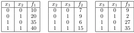
x1 x2 f1
0 0 10 0 1 20 1 0 35 1 1 40
x2 x3 f2
0 0 7 0 1 9 1 0 6 1 1 15
x3 x1 f3
0 0 9 0 1 2 1 0 27 1 1 35
Figure 1: Three Constraints of DCOP in Example 5
Gershman, Meisels, and Zivan 2009; Yeoh and Yokoo 2012) is a tupleD=hX,D,F,A, αiwhere
• X ={x1, . . . , xm}is a finite set of (decision)variables; • D={D1, . . . , Dm}is a set of finitedomains, where each
Diis the domain of variablexi∈ X;
• F ={f1, . . . , fp}is a finite set ofconstraints, where each
kj-ary constraintfj : Dj1 ×Dj2×. . .×Djkj 7→ R∪
{+∞}specifies thecostof each combination of values of the variables in itsscope; the scope of fj is denoted by
scp(fj) ={xj1, . . . , xjkj}; 3
• A={a1, . . . , an}is a finite set ofagents; • α:X 7→ Amaps each variable to an agent.
In the DCOP literature, the constraintsfjare also called ob-jective functionsorcost functions. We say that an agentai owns the variable xj ifα(xj) = ai. Each constraint inF can be eitherhard(i.e., some value combinations result in a utility of+∞and must be avoided), orsoft, (i.e., all value combinations result in a finite cost and need not be avoided). Given a constraint fj and a complete value assignment x (i.e., a value assignment for all variables), we denote with
xfj a partial value assignment fromxfor all variables in scp(fj). For simplicity, given two value assignmentsxand
x0, we writex = x0 whenever(1) if(x
i = di) ∈ x, then (xi =di)∈x0, and(2)conversely, if(xi =di)∈x0, then (xi = di)∈ x. Asolutionof a DCOP is a complete value assignmentx, and its correspondingtotal costis the evalua-tion of all cost funcevalua-tions onx. The goal of a DCOP is to find a cost-minimal solutionx∗= arg minx
Pp
j=1fj(xfj).
In this paper, we adopt asimplifying assumptionthat each agent owns exactly one variable. This assumption is a com-mon practice in the DCOP literature (Petcu and Faltings 2005; Gershman, Meisels, and Zivan 2009; Ottens, Dimi-trakakis, and Faltings 2012). Thus, without loss of general-ity, we assumeα(xi) = ai. It is relatively straightforward to generalize the ideas presented below to model a general DCOP, which allows agents to own multiple variables.
Example 5. Considering a DCOPD = hX,D,F,A, αi
where X = {x1, x2, x3}, D = {D1, D2, D3} in which Di = {0,1}withi ∈ {1,2,3},A = {a1, a2, a3}, andα
is defined asα(xi) = ai. Figure 1 exhibits the three con-straintsf1, f2, andf3betweenx1 andx2, betweenx2 and x3, and betweenx3andx1, respectively.
It is possible to see that the solution of D is the value assignment in whichx1 = x2 = x3 = 1 which yields the
minimal total cost of40 + 15 + 35 = 90.
We will now show how a DCOP can be encoded using an MCS-OP. We first specify the space of all solutions of a
3
DCOPD =hX,D,F,A, αiwithnagents (i.e.,|A| =n) as equilibria of an MCSMD0 = (C1, . . . , Cn)ofncontexts.
Each contextCicorresponds to the agentai ∈ A. For sim-plicity, we specifyCi=(Li, kbi, bri), for1≤i≤n, where: • Li is the logic of the Answer Set Programming (ASP) framework (Gelfond and Lifschitz 1991). We also use the extended syntax of logic programs such as choice atoms, aggregates, etc. that have been adapted and implemented in most ASP solvers.
• kbiconsists of a rule (assuming thatDi={d1i, . . . , dsi})
1{value(xi, d1i), . . . , value(xi, dsi)}1← (3)
Intuitively, the rule of the form (3) enforces the selec-tion of exactly one of the listed values (i.e.,value(xi, d`i) with1 ≤ ` ≤ s) to an answer set ofkbi. Furthermore,
value(xi, d`i)in an answer set ofkbimeans that the vari-ablexiis assigned the valued`i ∈Di.
• briconsists of bridge rules of the form
(Bfj(dj1,...,djkj))costfj(V) ← (j1 :value(xj1, dj1)),
. . . , (4)
(jkj :value(xjkj, djkj))
for each constraintfj (e.g.,scp(fj) ={xj1, . . . , xjkj})
such thatα(xj1) = ai, where for1≤`≤kj,dj` ∈Dj`
and V = fj(dj1, . . . , djkj). Intuitively, V is the cost
specified by the constraintfj with respect to the respec-tive value assignment of variables in scp(fj) that are given in the body of the bridge rule (i.e.,value(xj`, dj`)).
Thus, V ∈ R ∪ {+∞}. Note that bri will contain |Dj1| × |Dj2| ×. . .× |Djkj|bridge rule(s) for every fj
such that α(xj1) = ai. In (4), Bfj(dj1,...,djkj) is the uniquename of the respective bridge rule.
Given a solutionxof a DCOPDin whichxiis assigned valuedi∈Di(i.e.,xi=di) for1≤i≤n, let
E(x) = (S1, . . . , Sn)be a belief state where:
Si={value(xi, di)}∪ (5)
{costfj(V)|scp(fj) ={xj1, . . . , xjkj}, α(xj1) =ai,
V =fj(xj1=dj1, . . . , xjkj =djkj)} (6)
Furthermore, given a belief stateS = (S1, . . . , Sn)ofMD0 ,
we letA(S)be a (partial) value assignment in whichxi=di ifvalue(xi, di)∈Si. The next theorem relatesDandMD0 .
Theorem 2. LetDbe a DCOP andM0
Dbe its
correspond-ing MCS. We have:
• IfSis an equilibrium ofMD0 , thenx=A(S)is a solution ofD; and
• Ifxis a solution ofD, then,S=E(x)is an equilibrium ofMD0 .
To be able to model the cost-minimal solution of DCOP, we extend the MCSMD0 into an MCS-OPMD by adding
a set of cost-assignment bridge rules (i.e., cbri) to con-texts of MD0 . Formally, given a DCOP D let MD =
(C1, . . . , Cn)be an MCS-OP withCi= (Li, kbi, bri, cbri)
whereM CS(MD) =MD0 andcbriis:
cbri={Bfj(dj1,...,djkj)@V ← |Bfj(dj1,...,djkj)∈bri,
head(Bfj(dj1,...,djkj))≡costfj(V)} (7)
Intuitively, a cost-assignment bridge rule of the form (7) means that if the bridge rule Bfj(dj1,...,djkj) is applicable
and its head (e.g., costfj(V)) is added to the respective
knowledge base, then this bridge rule will incur a cost (e.g., a cost ofV).
By Definition 5 and cost-assignment bridge rules of the form (7), it is simple to derive Lemma 2 below. Let us re-mind that, given a belief stateSofMD,cMSD(cS, for short) is the cost impact ofMDinS.
Lemma 2. LetSbe an equilibrium ofMD. We have
cS =
X
costfj(V)∈S
V (8)
We also can conclude the next lemma to relatecSwith the total cost on value assignmentx=A(S).
Lemma 3. LetDbe a DCOP andMD be its
correspond-ing MCS-OP. Ifxis a solution ofDand S = E(x)is an equilibrium ofMD(see the second item of Theorem 2), then
cS = p
X
j=1
fj(xfj) (9)
The next theorem relates DCOPDand MCS-OPMD.
Theorem 3. LetDbe a DCOP andMDbe its
correspond-ing MCS-OP. We have:
• If S is a most preferred equilibrium of MD, then x =
A(S)is a cost-minimal solution ofD; and
• Ifxis a cost-minimal solution ofD, thenS =E(x)is a most preferred equilibrium ofMD.
To sum up, Theorem 3 means that one can use MCS-OP to model DCOPs, where the semantics of MCS-OP as most preferred equilibria are directly related to the semantics of DCOPs as cost-minimal solutions.
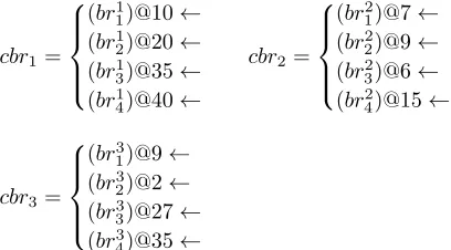
Example 6. The DCOPDin Example 5 can be modeled us-ing a MCS-OPMD = (C1, C2, C3)where withi∈ {1,2,3} Ci= (Li, kbi, bri, cbri)in which (for short, in the following we use predicate“val” instead of “value”):
kbi={1{val(xi,0), val(xi,1)}1←}
br1=
(br1
1)costf1(10)←(1 :val(x1,0)),(2 :val(x2,0)) (br1
2)costf1(20)←(1 :val(x1,0)),(2 :val(x2,1)) (br1
3)costf1(35)←(1 :val(x1,1)),(2 :val(x2,0)) (br1
4)costf1(40)←(1 :val(x1,1)),(2 :val(x2,1))
br2=
(br2
1)costf2(7)←(2 :val(x2,0)),(3 :val(x3,0)) (br2
2)costf2(9)←(2 :val(x2,0)),(3 :val(x3,1)) (br2
3)costf2(6)←(2 :val(x2,1)),(3 :val(x3,0)) (br2
4)costf2(15)←(2 :val(x2,1)),(3 :val(x3,1))
br3=
(br3
1)costf3(9)←(3 :val(x3,0)),(1 :val(x1,0)) (br3
2)costf3(2)←(3 :val(x3,0)),(1 :val(x1,1)) (br3
3)costf3(27)←(3 :val(x3,1)),(1 :val(x1,0)) (br3
cbr1=
(br1
1)@10←
(br1
2)@20←
(br1
3)@35←
(br14)@40←
cbr2=
(br2 1)@7←
(br2 2)@9←
(br2 3)@6←
(br24)@15←
cbr3=
(br31)@9← (br3
2)@2←
(br3
3)@27←
(br3
4)@35←
It is possible to see thatMDhas the most preferred
equi-libria:S= ({val(x1,1)},{val(x2,1)},{val(x3,1)})
Expressivity: MCS-OP vs. DCOP
The previous section shows that MCS-OP can model DCOP. For a researcher in the DCOP community, it raises the ques-tion whether the use of MCS-OP would bring any advan-tages over the DCOP formalization or it is just yet another way to formalize DCOP. This section answers this question by presenting a problem that can be straightforwardly for-malized using MCS-OP but not in DCOP.
Example 7. We extend Example 2 assuming thatC2 also
decides whether they go to their hotel by shuttle (s) or taxi (t). If they stay in Hilton, usings(resp.t) costs them$10 (resp.$30), and if they stay in Inn, usingsortcosts them $40or$30respectively.C2prefers the cheaper
transporta-tion because he will pay for this cost because it is not ac-counted to the total cost forC1andC2to travel together.
It is clear to see that since the cost of going to hotel is not accounted to the total cost, the most preferred group decision is the same as the one in Example 2 (i.e., selectbandi) and thus taking a taxi to go to Inn because it is cheaper than taking a shuttle. The total cost remains the same as$160.
Example 7 can be modeled using the MCS-OPM in Ex-ample 3, with the following modification:(i)L2 is answer
set optimization program (Brewka, Niemel¨a, and Truszczyn-ski 2003), and (ii) kb2 is extended with the two rules s > t←handt > s←i. Intuitively, the former rule states that ifC2stays inh, he prefersstot. The latter rule means
that if he stays ini, he prefersttos. It is possible to check that the most preferred equilibrium of this updated MCS-OP is({b},{i, t})that corresponds to the most preferred group decision mentioned above (i.e., selectb, iandt).
If we were to use DCOP to model Example 7, it is necessary to introduce three variables x1, x2, and x3 to represent the flight, hotel, and taxi, respectively.
Formally, a DCOP that may model Example 7 is D = h{x1, x2, x3},{D1, D2, D3},{f1, f2, f3, f4},{C1, C2}, αi
whereD1 = {b, e}, D2 = {h, i}, D3 = {s, t}, α(x1) = C1, α(x2) = C2, α(x3) = C2, and the four constraints f1, f2,f3, andf4are given in Figure 2. Intuitively,f1and f2represent the cost relation forx1(byC1) andx2(byC2),
respectively. Whilef3models the hard constraints between x1 andx2 (similar tobr1 andbr2),f4 represents the cost
relation betweenx2andx3(byC2).
x1 f1
e 50
b 100
x2 f2
h 120
i 60
x1 x2 f3
e h 0
e i ∞
b h ∞
b i 0
x2 x3 f4
h s 10
h t 30
i s 40
i t 30
Figure 2: Four Constraints of DCOP Modeling Example 7
It is possible to check that this DCOP D derives an un-expected cost-minimal solution (i.e., select e, h, and s) which yields the minimal total cost of $180. It is because the preferences of C2 on taking a taxi or a shuttle to the
hotel must be encoded as a constraint (i.e.,f4), and thus its
respective cost is accumulated to the total cost, deriving an unexpected minimal-cost solution. We believe that the lack of expressibility of the representation formalism of DCOP is the reason that prevents DCOP from successfully modeling the scenario in Example 7. MCS-OP is indeed more expres-sive than DCOP and could be useful in scenarios where some preferences among agents need to be considered locally and not be accounted for in the aggregation.
Related Work
To the best of our knowledge, MCS with preferences (MCSP), introduced in (Le, Son, and Pontelli 2015) and ex-tended in (Le, Son, and Pontelli 2018) is the most similar proposal to MCS-OP in that both approaches aim at defin-ing a preference order (or a qualitative comparison) among equilibria of MCSs. We therefore relate MCSP and MCS-OP in details before discussing others extensions of MCS.
MCSP assumes that the underlying logic of each context is a ranked logic, i.e., a logic with a preference order among its pairs of knowledge bases and belief sets. The preference order among equilibria of an MCSP is defined by pairwise combining the local preference orders. Specifically, an equi-libriumS = (S1, . . . , Sn)isstrongly(weakly) preferred to
another equilibrium S0 = (S01, . . . , S0n)if for every i, Si is strongly (weakly) preferred toSi0 with respect to the un-derlying ranked logic of contexti. An equilibrium is most strongly (weakly) preferred if there exists no other equilib-rium that is strongly (weakly) preferred to it. Thus, a most strongly (weakly) preferred equilibrium in MCSP is similar to a Nash equilibrium of a game for “personal” preferences among the contexts. Then, it is not an easy task to use MCSP in formalizing problems such as DCOP where the preference order often spans more than a single local context.
shows that MCS-OP can be used in scenarios where agents do have local preferences which, desirably, should not be considered in the aggregate preferences of the whole system. In this sense, MCS-OP provides a continuum from fully co-operative agents (as in MCS with a centralized controller) to non-cooperative or self-interested agents (as in MCSP).
Beside equilibrium semantics, (Brewka and Eiter 2007) proposedminimal/grounded equilibriaandwell-founded se-mantics for MCS. For the former, one can directly utilize our approach (i.e., assigning conditional cost to bridge rules) to derive the preferences among equilibria, and thus obtain the semantics of the most preferred minimal/grounded equilib-ria. Moreover, it is unclear how our approach could be used to derive the preference in the well-founded semantics, as it is defined using anantimonotoneoperatorγM(.).
Some significant extensions of the MCS framework have been recently introduced.Managed MCS(mMCS) (Brewka et al. 2011) allows applied bridge rules to also perform arbi-trary operations on context knowledge bases, e.g., deletion or revision operators.Reactive MCS(rMCS) (Brewka et al. 2018) and evolving MCS (eMCS) (Gonc¸alves, Knorr, and Leite 2014) are extensions of mMCS to allow changes of observationsover time. In order to model real-world situa-tions of multi-agent systems (MAS),DACMACS(Costantini and Gasperis 2015) integrates Data-Aware Commitment-based MAS and MCS where agents not only interact among themselves, but also consult external heterogeneous data-and knowledge-bases to extract useful information. Clearly, these extensions are not designed to derive the preference among their respective equilibria, sequences of equilibria, or runs. It is our belief that an integration of cost-assignment bridge rules in these frameworks can enhance them by al-lowing the determination of a best run (or most preferred equilibrium).
Other extensions of MCS have been proposed, where the introduction of a preference order requires more in-depth study and will be the subject of future work, e.g., preference order among supported equilibrium semantics in generalized MCS (Tasharrofi and Ternovska 2014), in operational-like semantics ofasynchronous MCS (Ellmau-thaler and P¨uhrer 2015), or in idealized runsemantics of streaming MCS(Dao-Tran and Eiter 2017).
Another related line of research is preference-based in-consistency managementin MCS. An MCS is inconsistent if it does not have an equilibrium; research has been done to analyze the inconsistency to identify themost preferred diagnoses(Eiter et al. 2014). A diagnosis of an MCS intu-itively is a pair of the set of all bridge rules that are either removed or set to be applicable in all belief states to make the MCS consistent. There are ways to accommodate pref-erences among diagnoses (see (Eiter and Weinzierl 2017)), and intuitively one can see that the most preferred equilib-rium ofM is an equilibrium ofM after being applied to the most preferred diagnosis. Different from using diagnoses, (Mu, Wang, and Wen 2016) proposed to use Preferential MCS(PMCS), which are stratified MCS based on predeter-mined partial ordering among contexts. From such ordering, to address the inconsistency, one may ask for amaximal con-sistent sectionas the semantics of PMCS. Compared to our
work in this paper, there is a significant difference: the works in inconsistency management are used to resolve MCS that do not admit an equilibrium, while in MCS-OP preference information is directly integrated into the semantics to select among existing equilibria.
We note that there have been attempts to extend the DCOP model. For example, Asymmetric DCOPs (Grinshpoun et al. 2013) allows different agents owning variables in the scope of a constraint can incur to different costs, given a fixed join assignment. Multi-Objective DCOPs (Marler and Arora 2004) are problems involving more than one objective function to be optimized simultaneously. However, these ex-tensions do not address the difficulty in modeling scenarios where some preferences among agents need to be considered locally and not be accounted for in the aggregation. MCS-OP could therefore be viewed as an alternative to DCMCS-OP that avoids this difficulty.
Conclusions and Future Works
We proposed Multi-context System for Optimization Prob-lems (MCS-OP), which associate each context with a set of cost-assignment bridge rules that assign conditional cost to its bridge rules. The preferences order among equilibria are determined by the total incurred cost of actually-applied bridge rules in the equilibria. We discussed the MCS-OP’s complexity and showed how to model DCOPs using MCS-OP to illustrate the contribution of this paper to both the MCS community and the DCOP community.
It is not difficult to see that cost-assignment bridge rules can be introduced to any of the existing MCS extensions (e.g., MCSP, mMCS, asynchronous MCS (Ellmauthaler and P¨uhrer 2015) and streaming MCS (Dao-Tran and Eiter 2017)). In other words, MCS-OP can be easily integrated with almost all of the MCS extensions and the notion of a most preferred equilibrium of such an extension can be de-fined as in the “Most Preferred Equilibria” subsection. For this reason, it would be interesting to investigate the inte-gration of MCS-OP into other extensions of MCS and their properties (e.g., as we have mentioned in the previous sub-section, the cost-assignment bridge rules could be useful in mMCS to identify the best runs). We also plan to investi-gate the use of a meta-reasoning transformation as in (Eiter and Weinzierl 2017), which implements a rewriting tech-nique, to select most preferred equilibria. Furthermore, as we have mentioned in the introduction, there is only a few systems for computing MCS that have been developed. On the other hand, many efficient and scalable systems for solv-ing DCOPs. As such, we also plan to investigate algorithms for computing MCS/MCS-OP that can take advantage of ap-proaches used in computing DCOP solutions.
Acknowledgments
References
Brewka, G., and Eiter, T. 2007. Equilibria in heterogeneous nonmonotonic multi-context systems. In Proc. of AAAI, 385–390.
Brewka, G.; Eiter, T.; Fink, M.; and Weinzierl, A. 2011. Managed multi-context systems. In Proc. of IJCAI, 786– 791.
Brewka, G.; Ellmauthaler, S.; Gonc¸alves, R.; Knorr, M.; Leite, J.; and P¨uhrer, J. 2018. Reactive multi-context sys-tems: Heterogeneous reasoning in dynamic environments. Artif. Intell.256:68–104.
Brewka, G.; Niemel¨a, I.; and Truszczynski, M. 2003. An-swer set optimization. InProc. of IJCAI, 867–872.
Costantini, S., and Gasperis, G. D. 2015. Exchanging data and ontological definitions in multi-agent-contexts systems. InProc. of RuleML.
Dao-Tran, M., and Eiter, T. 2017. Streaming multi-context systems. InProc. of IJCAI, 1000–1007.
Eiter, T., and Weinzierl, A. 2017. Preference-based inconsis-tency management in multi-context systems. J. Artif. Intell. Res.60:347–424.
Eiter, T.; Fink, M.; Sch¨uller, P.; and Weinzierl, A. 2010. Finding explanations of inconsistency in multi-context sys-tems. InProc. of KR.
Eiter, T.; Fink, M.; Sch¨uller, P.; and Weinzierl, A. 2014. Finding explanations of inconsistency in multi-context sys-tems.Artif. Intell.216:233–274.
Ellmauthaler, S., and P¨uhrer, J. 2015. Asynchronous multi-context systems. InAdvances in Knowledge Representation, Logic Programming, and Abstract Argumentation - Essays Dedicated to Gerhard Brewka on the Occasion of His 60th Birthday, 141–156.
Fioretto, F.; Pontelli, E.; and Yeoh, W. 2018. Distributed constraint optimization problems and applications: A sur-vey.J. Artif. Intell. Res.61:623–698.
Gelfond, M., and Lifschitz, V. 1991. Classical negation in logic programs and disjunctive databases. New Generation Comput.9(3/4):365–386.
Gershman, A.; Meisels, A.; and Zivan, R. 2009. Asyn-chronous forward bounding for distributed cops. J. Artif. Intell. Res.34:61–88.
Gonc¸alves, R.; Knorr, M.; and Leite, J. 2014. Evolving multi-context systems. InProc. of ECAI, 375–380.
Grinshpoun, T.; Grubshtein, A.; Zivan, R.; Netzer, A.; and Meisels, A. 2013. Asymmetric distributed constraint opti-mization problems. J. Artif. Intell. Res.47:613–647. Kumar, A.; Faltings, B.; and Petcu, A. 2009. Distributed constraint optimization with structured resource constraints. InProc. of AAMAS, 923–930.
Lass, R.; Kopena, J.; Sultanik, E.; Nguyen, D.; Dugan, C.; Modi, P.; and Regli, W. 2008. Coordination of first respon-ders under communication and resource constraints (Short Paper). InProc. of AAMAS, 1409–1413.
Le, T.; Son, T. C.; and Pontelli, E. 2015. Multi-context systems with preferences. InProc. of PRIMA, 449–466.
Le, T.; Son, T. C.; and Pontelli, E. 2018. Multi-context systems with preferences. Fundam. Inform.158(1-3):171– 216.
L´eaut´e, T., and Faltings, B. 2011. Coordinating logistics operations with privacy guarantees. InProc. of IJCAI, 2482– 2487.
Maheswaran, R.; Tambe, M.; Bowring, E.; Pearce, J.; and Varakantham, P. 2004. Taking DCOP to the real world: Effi-cient complete solutions for distributed event scheduling. In Proc. of AAMAS, 310–317.
Mailler, R., and Lesser, V. 2004. Solving distributed con-straint optimization problems using cooperative mediation. InProc. of AAMAS, 438–445.
Marler, R., and Arora, J. 2004. Survey of multi-objective optimization methods for engineering. Structural and Mul-tidisciplinary Optimization26(6):369–395.
McCarthy, J. 1987. Generality in artificial intelligence. Commun. ACM30(12):1029–1035.
Modi, P. J.; Shen, W.; Tambe, M.; and Yokoo, M. 2005. Adopt: asynchronous distributed constraint optimization with quality guarantees. Artif. Intell.161(1-2):149–180. Mu, K.; Wang, K.; and Wen, L. 2016. Preferential multi-context systems.Int. J. Approx. Reasoning75:39–56. Ottens, B.; Dimitrakakis, C.; and Faltings, B. 2012. DUCT: an upper confidence bound approach to distributed con-straint optimization problems. InProc. of AAAI.
Petcu, A., and Faltings, B. 2005. A scalable method for multiagent constraint optimization. InProc. of IJCAI, 266– 271.
Roelofsen, F., and Serafini, L. 2005. Minimal and absent information in contexts. InProc. of IJCAI, 558–563. Tasharrofi, S., and Ternovska, E. 2014. Generalized multi-context systems. InProc. of KR.
Ueda, S.; Iwasaki, A.; and Yokoo, M. 2010. Coalition struc-ture generation based on distributed constraint optimization. InProc. of AAAI, 197–203.
Yeoh, W., and Yokoo, M. 2012. Distributed problem solv-ing.AI Magazine33(3):53–65.
Zivan, R.; Glinton, R.; and Sycara, K. 2009. Distributed constraint optimization for large teams of mobile sensing agents. InProc. of IAT, 347–354.