Quantitative data analysis of ESAR data

(1)

Quantitative data analysis of ESAR data

N. Phruksahiran and M. Chandra

Professorship of Microwave Engineering and Electromagnetic Theory, Chemnitz University of Technology, Germany

Correspondence to: N. Phruksahiran ([email protected])

Abstract. A synthetic aperture radar (SAR) data processing uses the backscattered electromagnetic wave to map radar reflectivity of the ground surface. The polarization prop-erty in radar remote sensing was used successfully in many applications, especially in target decomposition. This pa-per presents a case study to the expa-periments which are paper-formed on ESAR L-Band full polarized data sets from Ger-man Aerospace Center (DLR) to demonstrate the potential of coherent target decomposition and the possibility of using the weather radar measurement parameter, such as the differ-ential reflectivity and the linear depolarization ratio to obtain the quantitative information of the ground surface. The raw data of ESAR has been processed by the SAR simulator de-veloped using MATLAB program code with Range-Doppler algorithm.

1 Introduction

Nowadays, SAR Technology has been continuously devel-oped by many researchers. Therefore, many benefits of po-larimetric SAR (PolSAR) by using the physically properties of scattering mechanisms in the polarization signature was found. This leads to many theories and applications in the field of target decomposition. The polarimetric decomposi-tion theorems can be classified into coherent and incoherent target decompositions which have each different advantage. The coherency decomposition deal with the scattering ma-trix, the incoherent decomposition is based on the coherency or covariance matrices. In addition to the full polarimetric SAR systems that transmit two orthogonal polarizations and record both received polarization, i.e., (hh, hv, vh, vv), where h and v denote the horizontal and vertical polarizations, re-spectively, there is the so-called dual-pol SAR modes, that consider only two linear polarizations, i.e., (hh,hv), (vh,vv) and (hh,vv). Another parameter of interest are the differen-tial reflectivity(Zdr)and the linear depolarization ratio(Ldr),

that can be used to process the weather radar data to obtain the qualitative measurements.

In this paper, SAR simulator was developed by using MATLAB program in order to process the experimental data from DLR with Range-Doppler processing algorithm. The processed full-polarized data was used to investigate the some potential of the coherent decompositions in SAR po-larimetry.

This paper is organized as follows. In Sect. 2 we intro-duce the basics of the target decomposition, and in Sect. 3 we explain the experimental data and the data processing. In Sect. 4, the simulation results are presented. Finally, Sect. 5 provides the conclusions.

2 Basics

In general, the radar image of SAR system presents the mag-nitude of each pixel which can be scaled to show the depth of the image, so that we can interpret it like the optical im-age. The visual analysis needs the correct perception of the observer to identify the targets on the ground. The target de-composition theorems are developed based on the wave po-larization basis to aim at providing such an interpretation.

The main categories of decompositions and parameter considered in this paper are the following: Pauli decompo-sition, differential reflectivity and linear depolarization ratio. 2.1 Pauli decomposition

(2)

[S]=

Shh Shv Svh Svv

(1)

=√a 2

1 0 0 1

+√b 2

1 0 0−1

+√c 2

0 1 1 0

+√d 2

0−j j 0

(2) The parametera, b, candd are complex quantities repre-senting, respectively, single or odd-bounce scattering, double or even-bounce scattering, 45◦ _{rotated double-bounce} scat-tering, and the anti-symmetric components of the scattering matrix, and are given by:

a =Shh√+Svv

2 (3)

b=Shh√−Svv

2 (4)

c=Shv√+Svh

2 (5)

d =jShv√−Svh

2 . (6)

In the case of the monostatic radar operation, it is assumed thatShv=Svh, and the Span value is given by:

Span= |Shh|2+2|Shv|2+ |Svv|2= |a|2+ |b|2+ |c|2 . (7) The color-coded representation with the basic colors (red, blue, green) can be used to recreate the image correspond-ing to the color-coded of each complex quantity.

2.2 Differential reflectivity and linear depolarization ratio

The differential reflectivity(Zdr)and the linear depolariza-tion ratio(Ldr)are commonly used in weather radar mea-surements. At the weather radar, the target volume is taken for analysis. The SAR system receives the reflected signals of ground targets and processes the data to the final image that represents the reflection properties of the ground.

The differential reflectivityZdr can be calculated in dB as the ratio of the reflectivity in horizontal polarizationShhand the reflectivity in vertical polarizationSvv by the following equation as shown by Yanovsky (2000):

Zdr=10·log₁₀Shh

Svv . (8)

The important information from theZdr value depends on the target structure. If Zdr is closely zero, the structure is sphere. The structure has the more length in horizontal axis when theZdr value is more than zero. Adversely, the Zdr value is less than zero then, the structure has the more length in vertical axis.

The linear depolarization ratioLdris one of the interesting ratios from measurement and is the fraction of refractivity

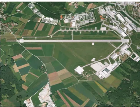
Fig. 1. Google Earth image of the test area.

between the co- and cross-polar radar signal channels by the following equation:

Ldr=10·log10 Svh

Shh . (9)

3 Experimental data and data processing

The experimental L-Band full polarized of Opairfield Test Site Area of Germany data set, which was used in this paper, is from the airborne ESAR flown by the German Aerospace Center (DLR), obtained on 20 February 2003. The terrain, as shown in Fig. 1, is a mixture of the flat surfaces, trees and buildings.

There are numerous SAR simulators for development of a radar system and radar processing. In this paper the range Doppler algorithm have been chosen to process the SAR raw data from ESAR.

The overview of the ESAR data signal processing with range Doppler algorithm and the target decomposition is shown in Fig. 2. The SAR simulator program was developed to read the binary raw data and to convert it to the two dimen-sion SAR matrices data in range and azimuth direction for the following data processing as shown by Cumming (2005).

(3)

Fig. 2. Functional block diagram of ESAR signal processing with range Doppler algorithm and target decomposition.

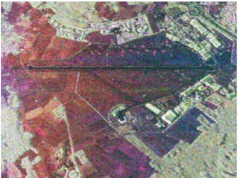
Fig. 3. Image data of hh-polarization channel from ESAR (DLR).

to the azimuth frequency axis. The azimuth compression is performed by using the matched filter function at each range gate. Then the processed data of the respective polarization channels are used for the purpose of target decomposition.

4 Results

This section presents the simulation results for the purpose of the alternative or supplement information of polarimetric SAR data to the existing target decomposition methods. 4.1 Image data

After digital signal processing, the four polarized data sets have been created in hh, hv, vh and hv polarization. The Im-age data can be shown with gray scale by using the difference of signal intensity from the target or the surface of interest. The signal intensity depends on the scattering properties of each target structure according to the polarization state of the SAR operation. In this paper, we used the Range-Doppler al-gorithm to process each SAR data channel, i.e., hh, hv, vh and vv, with the same system parameter and data processing in frequency domain.

Fig. 4. Pauli decomposition, the image is colored by blue for|a|2; red for|b|2; green for|c|2.

Figure 3 presents the image data of ESAR data set in hh polarization after the signal processing with Range-Doppler algorithm with sub-aperture length in azimuth direction and without the multi-look processing to reduce the speckle noise which arises in SAR because the relative phase of individual scatters. So that we can get and use the original image data set to test the target decomposition method and quantitative parameter of radar image as following.

4.2 Pauli decomposition

In general, the Pauli decomposition provides a tool for im-age classification that has been well known for decades in radar remote sensing communities. The three component of the Pauli composition are represented with color-coded blue, |a|2; red,|b|2and green,|c|2, respectively. Figure 4 presents the corresponding color-coded Pauli reconstructed image.

If we compare Fig. 1 with Fig. 4, we can realize the Pauli signatures of each part on the test area. The area on the right above is the residential area with many houses, which have the structure of dihedral, the red color dominates. The run-way and street areas are presented by dark tone. It is clear to see that the forest area is in green. The areas in which the scattering mechanisms are simultaneously presented are shown with white. The different colors show that each polar-ization provides other information.

4.3 Differential reflectivity and linear depolarization ratio

(4)

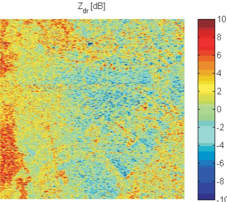
Fig. 5. Simulation results ofZdrof test site area in dB.

4.3.1 Zdrvalues

Figure 5 presents the simulation results of differential reflec-tivity by using the reflecreflec-tivity difference between hh- and vv polarization SAR operation. The values are shown in dB with the value range [−10,10].

By using the color-coded according to theZdrvalues, one can see that there are different shades of each area on the image. When considered as a whole, it can be seen that the smooth area has theZdrvalues less than zero, the blue color dominates. The another area which consists of a building or area of forest has theZdrvalues more than zero, the red color dominates. In the area of forest and building, there is not much of difference from each other. By using the differential reflectivity, we can see and image the contour of the ground structure and it can be separated the flat area from the area with forest and building.

4.3.2 Ldrvalues

Figure 6 presents the simulation results of linear depolariza-tion ratio by using the reflectivity difference between vh- and hh polarization SAR operation. The values are shown in dB with the value range [−10,10].

The values of linear depolarization ratio as shown in Fig. 6 have the uneven distribution. But one can indicate that the values ofLdr are less than zero for the smooth area and the values ofLdrare more than zero for the area with buildings. 4.3.3 AppliedZdrvalues

In Fig. 5, we have defined a continuous change of color-coded of the differential reflectivity values to compare the values obtained from the experiments, so that we can see the approximately difference between each type of surface.

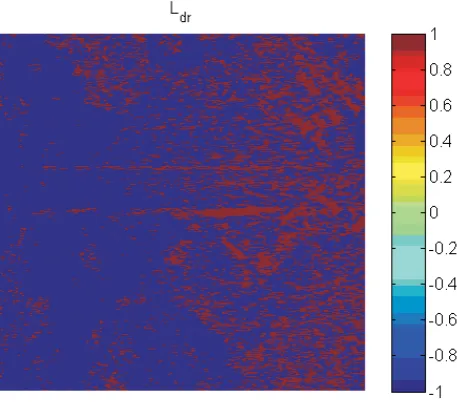
Fig. 6. Simulation results ofLdrof test site area in dB.

Fig. 7. AppliedZdrvalues with−1 and 1.

Figure 7 presents the simulation results of differential re-flectivity by using the rere-flectivity difference between hh- and vv polarization SAR operation. The values are shown with −1 and 1 for theZdrvalues which are less than zero and the Zdrvalues which are equal or more than zero, respectively.

(5)

Fig. 8. AppliedLdrvalues with−1 and 1.

variableZdrare equals to−1 and if the surface is not smooth, the value of the variableZdrare equals to 1.

4.3.4 AppliedLdrvalues

The same approach to the display the appliedZdr values in Fig. 7 has been used to present the simulation results of the linear depolarization ratio from the Fig. 6, so that the values in the Fig. 8 are shown with−1 and 1 for the Ldr values which are less than zero and theLdrvalues which are equal or more than zero, respectively.

The benefit of this approach is the values of Ldr in the area with large buildings. By comparing the location of the building in Fig. 1 one can see the border of the building in Fig. 8 at the same location as well.

4.4 Comparison of appliedZdr values and appliedLdr values

By comparing the values of the applied differential reflec-tivity in Fig. 7 and the applied linear depolarization ratio in Fig. 8 at each area, it can be divided in four cases as follow-ing:

1. +Zdrand+Ldr: the areas that may have a positiveZdr values and positiveLdrvalues are larger building. 2. +Zdr and −Ldr: in the vicinity of the houses or

vil-lages with a characteristic dihedral structure, the Zdr may have a positive values but theLdr may have neg-ative values.

Zdr Ldr

mine exactly what are the surface characteristics and the kind of target.

4. −Zdrand−Ldr: the simulation results also indicate that the flat area and fields may have the negative values of ZdrandLdr.

5 Conclusions

In the first part of this paper, we have provided a short review of Pauli decomposition, differential reflectivity and linear de-polarization ratio. The SAR simulator was developed to pro-cess the polarimetric raw data set of ESAR from DLR with range Doppler algorithm. The findings indicate that some pa-rameter which was used to evaluate weather data set such as differential reflectivity and linear depolarization ration can be used for the decomposition purpose in SAR radar remote sensing and they are considered as a useful addition to the decomposition theorems. Since the simulation results are ob-tained with only one polarimetric test data set, the interpre-tation and the conclusion have particular limiinterpre-tation. Further work will also include the development of improved simula-tion method for a better interpretasimula-tion of the various target decompositions, in particular the alternative measurement parameter, e.g., the differential reflectivity and the linear de-polarization, as an additional feature of the target decompo-sition method in SAR image data.

Acknowledgements. The authors would like to thank Al-berto Moraira of DLR, Germany, for providing the full polarimetric ESAR data set which was used in EU project AMPER.

References

Cumming, I. G. and Wong, F. H.: Digital Processing of Synthetic Aperture Radar Data Algorithms and Implementation, Artech House, Norwood, 2005.

Klausing, H. and Holpp, W.: Radar mit realer und synthetischer Apertur Konzeption und Realisierung, Oldenbourg, Muenchen, 2000.

Lee, J. S. and Pottier, E.: Polarimetric Radar Imaging from Basics to Applications, CRC Press, Boca Raton, 2009.