R E S E A R C H
Open Access
Exploiting spectro-temporal locality in deep
learning based acoustic event detection
Miquel Espi
*, Masakiyo Fujimoto, Keisuke Kinoshita and Tomohiro Nakatani
Abstract
In recent years, deep learning has not only permeated the computer vision and speech recognition research fields but also fields such as acoustic event detection (AED). One of the aims of AED is to detect and classify non-speech acoustic events occurring in conversation scenes including those produced by both humans and the objects that surround us. In AED, deep learning has enabled modeling of detail-rich features, and among these, high resolution spectrograms have shown a significant advantage over existing predefined features (e.g., Mel-filter bank) that compress and reduce detail. In this paper, we further asses the importance of feature extraction for deep learning-based acoustic event detection. AED, based on spectrogram-input deep neural networks, exploits the fact that sounds have “global” spectral patterns, but sounds also have “local” properties such as being more transient or smoother in the time-frequency domain. These can be exposed by adjusting the time-frequency resolution used to compute the spectrogram, or by using a model that exploits locality leading us to explore two different feature extraction strategies in the context of deep learning: (1) using multiple resolution spectrograms simultaneously and analyzing the overall and event-wise influence to combine the results, and (2) introducing the use of convolutional neural networks (CNN), a state of the art 2D feature extraction model that exploits local structures, with log power spectrogram input for AED. An experimental evaluation shows that the approaches we describe outperform our state-of-the-art deep learning baseline with a noticeable gain in the CNN case and provides insights regarding CNN-based spectrogram characterization for AED.
Keywords: Acoustic event detection; Local spectro-temporal characterization; Feature extraction; Time-frequency resolution; Convolution neural networks
1 Introduction
In the context of conversational scene understanding, most research is directed towards the goal of automatic speech recognition (ASR), because speech is arguably the most informative sound in acoustic scenes. For humans, non-speech acoustic signals provide cues that make us aware of the environment, and while most of our atten-tion might be dedicated to actual speech, “non-speech” information is critical if we are to achieve a complete understanding of each and every situation we face. More-over, this information is implied by the speakers, and so they actively or passively neglect mentioning certain concepts that can be inferred from their location, the cur-rent activity, or event occurring in the same scene. For instance, in a situation where two speakers are watching a
*Correspondence: [email protected]
NTT Communication Science Laboratories, NTT Corporation, 2-4, Hikaridai, Seika-cho, Keihanna Science City, 619-0237 Kyoto, Japan
sports game, most of the spontaneous speech utterances are very likely to be related to sports, and ASR could bene-fit from having such topic knowledge in advance [1]. On a smaller scale, if we hear a door opening, we usually assume that somebody has left or entered the room. Having access to such information in an automated manner can enhance the performance of ASR, diarization, or source separation technologies [2].
Acoustic event detection (AED) is the field that deals with detecting and classifying these non-speech acoustic signals, and the goal is to convert a continuous acous-tic signal into a sequence of event labels with associated start and end times. The field has attracted increasing attention in recent years including dedicated challenges such as CLEAR [3], and recently D-CASE [4], with tasks involving the detection of a known set of acoustic events happening in a smart room or office setting. In addi-tion, AED applications range from rich transcription in speech communication [3, 4] and scene understanding
[5, 6], to being a source of information for informed speech enhancement and ASR. Gaining access to richer acoustic event classifiers could effectively support speech detection and informed speech enhancement [2] by pro-viding the system with details about what kind of noise surrounds the speakers, besides the obvious benefits of richer transcriptions.
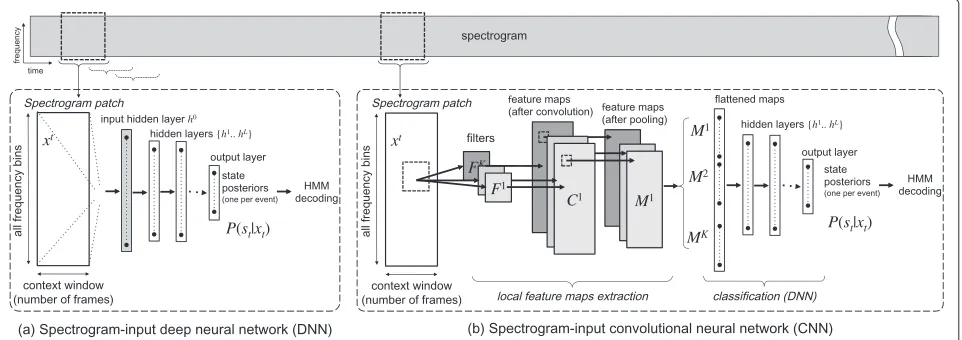
Recently, we have seen the potential of directly modeling the real spectrogram in AED in studies such as [7, 8]. The idea is that a detail-rich input such as a high reso-lution spectrogram is sparse enough to deal with com-plex scenarios with overlapping sounds. This comcom-plexity does not appear only in the frequency domain, but also in the form of a wide range of temporal structures. In [8] (Fig. 1a), the spectrogram patch concept is used to describe a model that receives an input including a con-text of frames from a spectrogram. This is rather typical in deep learning these days, but it is stressed here since a suf-ficient amount of short-time temporal structure regarding sounds can be packaged if the context is wide enough. This approach is possible given the ability of DNNs to model such a high dimensional input. This contrasts with traditional approaches in which the classifier models pre-defined acoustic features (e.g., MFCC, or Mel-filter banks) [9, 10], which compress and neglect details that we actu-ally need. Espi et al. [8] succeeds in modeling spectro-gram patches input as a whole, i.e.; it learns features that describe “globally” a short-time spectrogram patch. How-ever, this dismisses important properties of sounds (e.g., stationarity, transiency, burstiness, etc.), a taxonomy that could also help to model acoustic events.
This concept was considered in [10] by combining fea-tures extracted using multiple spectral resolutions, which resulted in better classification accuracy compared with standard single spectral scale features. This study exploits “local” as opposed to “global” characterization of the spectrogram. Such local properties, are also observable
at low feature levels (i.e., small and local subsets of adja-cent time-frequency bins), since they are local in the spectro-temporal domain.
This paper further investigates the importance of both using the real spectrogram as a feature and achiev-ing a proper characterization exploitachiev-ing spectro-temporal “locality”. We do this by exploring and comparing two approaches in parallel: first, augmenting the input with multi-resolution features and therefore dealing with the locality outside the model, and second, exploiting the locality with a model that integrates that concept, all within the context of deep learning.
The main contribution of this paper relates to the fact that while existing works rely on features that are defined and crafted to fit certain characteristics of sounds, deep learning is powerful enough to learn features by itself when the appropriate architectures are in place. This work is not novel in terms of using deep learning for acoustic event detection as this is already familiar in ASR [11], and we are starting to see it in acous-tic event detection as well [12]. What these studies do not do is truly exploit the feature learning ability of deep learning and use custom crafted features downsam-ple and focus on specific properties of certain sounds. Here, we show how, with the appropriate architectures, deep learning models can learn features directly from a naive feature (i.e., the log power spectrogram in this work).
The paper continues with Section 2, which addresses the importance of spectro-temporal locality, and intro-duces standard notions related to the deep learning frame-work in the context of AED. Section 3 describes the first approach combining multiple resolution spectrogram-input DNN classifiers, thus dealing with locality outside the model. In Section 4, the spectrogram-input con-volutional neural network (CNN) [13, 14] is discussed, reporting the results of our experimental evaluation in
Section 5. Section 6 discusses the results and the insights we obtained, concluding the paper with Section 7.
2 Conventional method and problem statement This section describes a spectrogram input deep learning AED baseline along with its limitations and the motiva-tions that lead to the feature extraction strategies in this study. It also includes a description of the spectrogram input CNN framework that is evaluated later on.
2.1 Deep learning-based acoustic event detection In [8], we can find an AED approach that directly mod-els log spectra patches rather than pre-designed features using deep neural networks (DNN). To better charac-terize sounds that are quite different from speech, a high-resolution spectrogram patch (a window of spectro-gram frames stacked together) is directly used as input shown in Fig. 1a. This ensures that the input feature is embedded with enough time-frequency detail. But, mean-ingful features still need to be obtained from such a high-dimensional input. Restricted Boltzmann machines (RBMs) [15] provide a useful paradigm for accomplishing this, since they are unsupervised generative models with great high-dimensional modeling capabilities, and allow the model to learn features from data. Moreover, RBMs form the basis of current state-of-the-art deep neural net-works (DNNs) [16], allowing seamless integration into the DNN framework.
The resulting model consists of a chain of RBM feature-extraction layers trained in cascade by using spectrogram patches as the input to the first layer and the output of each layer as the input to the next layer. Pretrained layers are then stacked together, with a softmax layer on top that has an output node for each output state in the recognizer, to form a deep neural network following standard deep learning techniques [16]. The entire network is trained to estimate state posteriors (one state per acoustic event), which will be decoded later as a hidden Markov model (HMM) forming what we know as a DNN-HMM. Please see [8] for more details.
2.2 Importance of spectro-temporal locality
The model we described above provides excellent per-formance, yet its main advantage is also a weakness, and this forms the underlying idea of this paper. It is because acoustic events have specific spectro-temporal shapes that DNNs are capable of characterization and classification with significant levels of robustness. How-ever, these spectro-temporal shapes are global, meaning that the DNN learns to model entire spectrogram patches. That is, the input layer learns weights that describe com-plete spectrogram patches. In a way, we can say that DNNs are able to learn a “global” characterization of an acoustic event. But that is only one side of the acoustic scene. While
sounds can be defined globally, a more abstract taxon-omy can also be defined resulting in properties such as stationarity and transiency, i.e., a “local” characterization. In the spectrogram domain, “local” refers to the con-cept of locality in time-frequency bins, and, with the deep learning model described in the previous subsection as the starting point, we approach this in two different ways: outside the model and with a model that integrates local characterization.
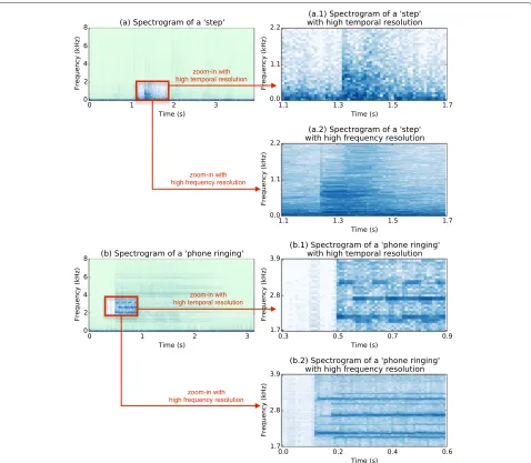
The first approach arises from observing the way in which different spectral resolutions show different infor-mation [10]. Figure 2 reveals that there are differences with regard to the information shown by different spec-tral resolutions. This is caused by the trade-off between time and frequency resolution. That is, increasing the frame length for computing the spectrum reduces the time resolution. On the other hand, this increases the fre-quency resolution. While this allows access to finer detail in the frequency axis, the risk arises of missing low-energy sounds such as “steps”. Conversely, with a shorter frame length, the time resolution increases, thus reducing the frequency detail, and potentially weakening the character-ization of sounds with specific frequency-wide patterns such as a “phone”, or a “door slam”. In summary, looking at different spectral resolutions simultaneously could yield some benefits in terms of performance.
The work reported in [10] exploits this by separating the acoustic signal into components based on different spectro-temporal scales, but again, these scales are hand-crafted, and further processing is used to downsample the feature resolution using MFCCs as features. We can now use multiple spectrograms with multiple resolutions directly as features thanks to the ability of deep architec-tures to model high-dimensional inputs.
The second approach is intended to integrate the spectro-temporal locality in the model itself. High-resolution spectrogram patches are expected to embed enough information about spectral and temporal struc-tures to model complex sounds. And, if this is exploited for “global” characterization, it can also be exploited for “local” characterization. Rather than having a fully con-nected input layer as in the DNN approach, a layer that only connects a local subset of time-frequency bins to each node of the hidden layer could exploit the concept of locality. Moreover, if the weights locally connecting input and hidden nodes are shared throughout the layer, the model can potentially learn features regarding station-arity, transiency, etc. CNNs do exactly this, and that is what makes them the ideal candidate for our integrated approach.
Fig. 2Magnified log power spectrogram regions for “steps” (a) and “phone ring” (b) sounds for high-time resolution (10 ms frame length, (a.1) and (b.1)) and high-frequency resolution (90 ms frame length, (a.2) and (b.2))
applications [17–19] besides computer vision, provide the means to extract local features from the spectro-gram itself. The convolution of relatively small-sized filters over a spectrogram patch makes it possible to learn local feature maps (convolution is only per-formed with adjacent bins in time and frequency, i.e., local).
CNNs consist of a pipeline of convolution-and-pooling operations followed by a multilayer perceptron, namely a deep neural network. CNNs are tightly related to the concept of feature extraction, modeling not just the input as a whole, but also independent local features in an integrative manner. The entire model is then globally con-structed by jointly training the convolutional and DNN
architectures as a whole using back-propagation (see Fig. 1b for an overview).
Spectrogram input CNNs exploit time-frequency local correlation by enforcing local connectivity patterns between neurons of adjacent layers. The input hidden units to the DNN part of the model (Ck, and Mk after pooling) are connected to a locally limited subset of units in the input spectrogram patch and are contiguous in time and frequency. Each filterFkis also replicated across the entire input patch forming a feature map, which shares the same parametrization (i.e., the same weights and bias parameters).
Ckare obtained from a spectrogram patch inputxtwith a linear filterFk of shapeS×S, adding a bias termbk, and applying a non-linear function,
Cijk=tanh
S m=1 S n=1 Fmnk xt
i+m−S
2
,j+n−S
2
+bk
(1)
wherextω,τrefers to the bin in the frequency indexωand frame indexτ, in patchxt. Max-pooling is then applied following a specific shapeP1×P2, which we have chosen
to obtain the feature mapMk,
Mkij=maxC(kiP
1:(i+1)P1),(jP2:(j+1)P2)
(2)
where P1 and P2 refer to pooling along frequency and
time, respectively (e.g., 1 × 1 pooling scheme is equiva-lent to no pooling). The pooling stage has no parameters, and therefore, there is also no learning.
The rest of the CNN architecture consists of fully con-nected layers of hidden nodes with sigmoid activations, which receive a flattened concatenation of all the feature maps M1· · ·MK as the input. Further details can be found in [13, 14].
3 Exploiting locality with multiple resolution spectrograms
Given the differences between acoustic events in terms of time and frequency resolution, we can assume that spectrogram-input AED systems are dependent on the resolution with which the spectrogram was computed. Figure 2 shows a magnified region of two acoustic events, “steps” and a “phone ringing” , with high-time resolution (top), and high-frequency resolution (bottom). Observing the high time resolution spectrogram (Fig. 2a.1, b.1), we can recognize onsets, transient sounds, and low-energy signals without great effort. This does not happen with high-frequency resolution (Fig. 2(a.2, b.2), but we have more detailed access in the frequency axis. This trade-off between time and frequency resolution is because the frame length influences the shape of the time-frequency bins in a spectrogram, and this shape influences the amount of detail on each axis. The ability to able to observe the spectrogram with a much wider shape that covers both long time and frequency regions simultane-ously could reveal much richer information.
In summary, the multi-resolution approach consists in a set multiple single-resolution DNN classifier working in parallel for the same task. The parallel output of this rec-ognizer is then combined using the scheme presented in subsection 3.1. As the presented approach includes sup-port for output of multiple event labels simultaneously, subsection 3.2 addresses why and how this compares with other single output models.
3.1 Combination scheme
We propose a simple combination scheme to merge the outputs of multiple single-resolution AED systems work-ing in parallel. The scheme combinwork-ing multiple spectral resolutions is as follows (see Fig. 3):
1. First, using a development set, we learn which single-resolution AED systemSrworks better with
each of the acoustic events in the task.
2. Multiple single-resolution recognizers, such as that described in subsection 2.1{S10,· · ·Sr· · ·SR}, each
working with a different spectral resolutionr (e.g.,
r=10ms frame length) provide output labels in parallel.
3. Then, each output will be filtered so that only the optimal set of eventsErfor resolutionr is selected, as
we have previously learned with a development set. 4. The final output is obtained by merging repeated
labels and/or removing the label “silence”, if there is another label already, on a frame-wise basis.
This is rather a simple approach, but we could draw conclusions from it.
3.2 On event overlapping and output of multiple labels The combination scheme described above allows the out-put of multiple labels on each frame. In other words, it considers the overlapping of acoustic events as long as those events are not assigned to the same single resolu-tion classifier. From a real world perspective, this is more realistic. In terms of performance, this can indeed result in an improvement of the performance as more events can be detected. For instance, a phone can ring while some-body is typing on a keyboard. However, in the proposed architecture, each of the single resolution classifiers target all events, and the results are filtered at the output of the classifier to allow only the labels for which each single res-olution classifier works better. In this way, this system can be compared to systems that only output a single label at each frame.
Moreover, even considering the previously described situation where a phone rings in the presence of a key-board typing sound, these non-speech events are still sparse enough in time to allow a single event classifier to recognize both properly, as a sequence of keyboard-phone events. For a further discussion of this topic, the reader can refer to [20], which presents different possible metrics for strongly polyphonic environments.
4 Exploiting locality with a spectrogram patch input CNN model
Fig. 3Multi-resolution spectrogram patch input classifier and label stream combination overview
example of spectrogram input CNN behaves with acoustic events.
4.1 AED specific considerations
CNN’s most important advantage is the ability to learn local filters from 2D inputs, and that is the motiva-tion behind using them to learn local maps from time-frequency patches. While in images this accounts for figure corners, edges, and so on, such filters are also mean-ingful when the inputs are spectrogram patches. Finding local features that highlight continuity in time, continu-ity in frequency, or other more fluctuating local patterns, allow the model to unfold a single spectrogram into many local feature maps and perform classification over.
4.2 Spectrogram-patch-input CNN
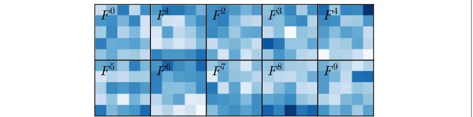
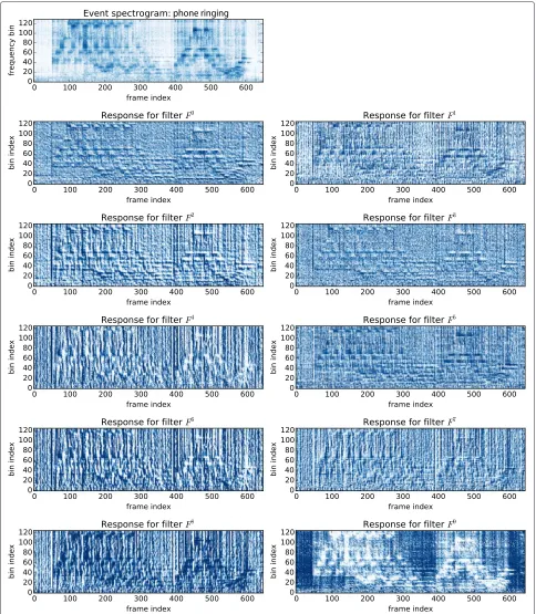
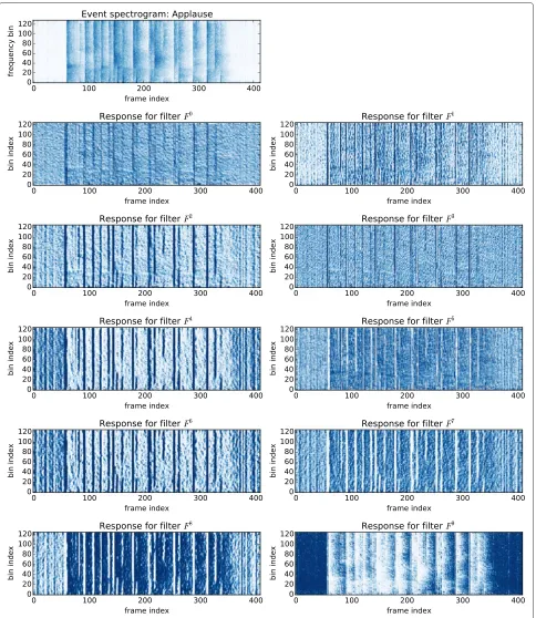
The principle of CNNs for replicating convolution filters as described in subsection 2.3 allows features learned by the model to be detected regardless of their position in time or frequency. This directly relates to the fact that we are not learning event-dependent features, but rather use-ful local filters that reveal more independent aspects of sounds. Figure 4 shows some of the filters learned dur-ing the experiments. For instance, maps for filters such as
F3orF4react very lightly to the sound of applause show-ing that they are not focused on transiency, while others such as F2, F4, F6, F8, andF9 do have quite noticeable
responses. The case of a phone ringing is more complex as onsets and stationary notes both appear, and this causes many convolution maps to activate in different ways to highlight different properties.
It would be interesting to see how these filters and their responses compare with other standard projection techniques used to enhance data such as PCA or LDA. However, this would require a way of ordering the filters and finding their equivalent filters between each CNNs and existing projection methods. We consider this to be worth exploring in the near future.
5 Experiments and results
As two approaches are being introduced in this paper, the models have been evaluated from two points of view:
• We evaluate how different parameters affect the multi-resolution and CNN approaches.
• We compare best scores for these with a
state-of-the-art DNN using a baseline based on [8].
This section presents the datasets, the setup parameters we used, and the evaluation results.
5.1 Datasets and front-end
The proposed approaches have been tested against the acoustic event recognition task in CHIL2007 [3], a
database of seminar recordings in which twelve non-speech event classes appear in addition to non-speech: applause (ap), spoon/cup jingle (cl), chair moving (cm), cough (co), door slam (ds), key jingle (kj), door knock (kn), keyboard typing (kt), laugh (la), phone ring (pr), paper wrapping (pw), and steps (st). This database con-tains three AED-related datasets which we have used for this evaluation: a training dataset called FBK that con-tains only isolated acoustic events without the presence of any speech, adevelopmentdataset that contains meet-ings in a similar manner to those in the evaluation dataset, and atestdataset that contains seminar recordings where speech and acoustic events appear in a natural manner and overlapping at times (60 % of the events reportedly overlap with speech in the test set [3]). Each dataset con-sists of 1.65, 3.27, and 2.55 h fortraining,development, and
test, respectively.
Additionally, to deal with the case where speech over-laps with acoustic events, we need such training data to have the neural network learn to discriminate in such a situation, and following the approach in [8], we have arti-ficially augmented the training dataset to contain speech-overlapped data by adding publicly available speech from AURORA-4 [21]. This is added by taking a random chunk of speech from the speech dataset and adding it to the isolated events dataset in different signal-to-noise ratios (SNR), where thesignalis the non-speech acoustic event and the noise is the speech that corrupts the targeted acoustic event. A total of eleven SNR conditions were gen-erated: -9, -6, -3, 0, 3, 6, 9, 12, 15, and 18 dB, andclean(no speech noise added).
The front-end consists of computing the log power spectrum and a frame basis, and stacking consecutive frames together as a two-dimensional feature. For CNNs, the log power spectrogram was computed using 10 ms frames with a 10 ms shift, which performed the best. For multi-resolution DNN, the frame lengths were 10, 20, 30, 40, 50, and 60 ms, with a 10-ms shift for all of them. The input into the neural networks was normalized to remove any variance.
5.2 Setup parameters
CNNs add more parameters to the typical deep model, and therefore, we have designed a broad set of experi-ments1to learn how these parameters affect the perfor-mance. All settings are summarized in Table 1.
CNN models have one convolution layer and four fully connected layers with 512 nodes each, while the DNN-only models have a first hidden layer with 1024 nodes to deal with the input and four hidden layers with 512 hid-den nodes each. We also compared the performance of the CNN settings with a DNN-only spectrogram-patch-based AED as described in subsection 2.1. Both CNN-based and DNN-only models were trained for 500 epochs.
Table 1Experimental setup parameters
Deep neural networks settings
FFT resolutions 10 ms (129 bins), 20 ms (257 bins)
(multi-resolution) 30 ms (257 bins), 40 ms (513 bins)
50 ms (513 bins), 60 ms (513 bins)
Patch lengths 10, 20, and 30 frames
Convolutional neural networks settings
Filter shapes (CNN) 5× 5, 7× 7, 9× 9 (bins×frames)
Number of filters (CNN) 10, 20, and 40 filters
Pooling (CNN) 1×1 (no pooling)
2× 1 (frequency pooling)
1× 2 (time pooling)
2× 2 (both axes)
The goal of this work is to compare the feature learning ability of convolutional (CNN) and fully connected layers (DNN), and that is why the compared models have the same architectures except for the first hidden layer. This allows us to fairly compare the spectrogram-modeling capabilities of both types of layers. The reader can refer to recent studies such as [12] in which the number of convolutional layers is adequately evaluated.
5.3 Multi-resolution results
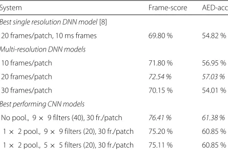
Table 2 compares the two metrics: frame-score (per-centage of correctly classified frames), as in Fig. 7, and AED-accuracy which is the event-wise f-measure between precision and recall. Overall results confirmed that even a simple combination approach provided a significant clas-sification score improvement over the best performing single-resolution DNN. This indicates the relevance of time-frequency resolution.
Looking at event-wise results with the best spectro-gram patch length (20 frames) as shown in Table 3, we compared the performance of the AED described sub-section 2.1 for several spectral resolutions (spectrum
Table 2AED evaluation results with the “test” set
System Frame-score AED-acc
Best single resolution DNN model[8]
20 frames/patch, 10 ms frames 69.80 % 54.82 %
Multi-resolution DNN models
10 frames/patch 71.80 % 56.95 %
20 frames/patch 72.54 % 57.03 %
30 frames/patch 70.15 % 54.01 %
Best performing CNN models
No pool., 9× 9 filters (40), 30 fr./patch 76.41 % 61.38 %
1×2 pool., 9× 9 filters (20), 30 fr./patch 75.20 % 60.85 %
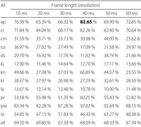
Table 3Resolution-event-wise results (frame-score %) for the best performing spectrogram patch size (20 frames/patch) DNN-only model
AE Frame length (resolution)
10 ms 20 ms 30 ms 40 ms 50 ms 60 ms
ap 76.39 % 65.39 % 66.32 % 82.65% 69.90 % 72.85 %
cl 71.84 % 84.04% 68.17 % 62.26 % 62.40 % 70.64 %
cm 31.59 % 35.71 % 33.73 % 30.98 % 44.00% 23.62 &
co 36.97% 27.82 % 27.49 % 17.09 % 21.58 % 29.97 %
ds 29.70 % 16.92 % 17.76 % 11.62 % 38.74% 21.66 %
kj 12.90 % 11.46 % 14.64 % 12.70 % 17.11% 13.66 %
kn 49.66 % 27.08 % 37.03 % 66.89% 44.57 % 23.55 %
kt 38.37% 27.97 % 26.98 % 27.29 % 32.61 % 28.59 %
la 13.67% 12.14 % 12.48 % 10.78 % 10.90 % 11.48 %
pr 53.58 % 55.98 % 51.35 % 60.25% 55.43 % 52.82 %
pw 83.34 % 82.28 % 87.28 % 92.02% 92.69 % 88.15 %
st 54.85 % 47.15 % 51.83 % 46.43 % 63.27% 48.38 &
all 69.20 % 69.80% 67.34 % 68.09 % 68.33 % 67.34 %
frame length) between 10 and 60 ms to determine its importance.
The first conclusion is that the best performing resolu-tion overall is not the best resoluresolu-tion for each and every acoustic event class separately. In general, and consis-tent with previous assumptions, certain low-energy events such as “keyboard typing” are better tracked with short frame resolutions, whereas long frames perform better for a “door slam” (50 ms). This is also the case with “applause” (40 ms), which has a very similar structure in the fre-quency domain. On the other hand, with events such as “chair move” , switching the frame length seems to have almost no effect on performance. Other sounds such as a “laugh” perform in various ways with no strong trend.
5.4 CNN results
The results are shown in Fig. 7, and the top scores are sum-marized for ease of comparison in Table 2. At first sight, the first conclusion is that we are able to achieve better performance than any DNN-only model (Table 2).
Figure 7 also provides some insights into CNN-based AED performance. The best performance came from the longest spectrogram patch configuration (Fig. 7a). Regarding the convolution filters, the results indicate that more filters provide better performance (Fig. 7b), and filter shapes covering smaller regions provide better per-formance on average (Fig. 7c), but the actual best score was obtained with a wide filter (Table 2). As for pooling, the general conclusion is that the effects are different for pooling along frequency and pooling along time (Fig. 7d). However, the results do show that performance degrades visibly when frequency pooling is included.
6 Discussion
6.1 Comparing multi-resolution input and CNN-based AED Conceptually, the multi-resolution DNN and the CNN approaches travel in different directions. Multi-resolution analysis approaches the issue of characterizing spectro-temporal locality outside the model, while the CNN approach itself exploits local features. These approaches are not mutually exclusive but complementary. While CNN performs better than combining resolutions, it is not hard to imagine in the near future a deep model in which parallel working convolution-and-pooling layers receive spectrogram patches of the same signal with different spectral resolutions, and where their outputs are stacked and fed to the DNN part of the CNN. The question then is if the potential gain is worth the cost.
6.2 Convolution filters
When we look at a specific example of the filters obtained for a simple CNN configuration (Fig. 4) the convolved maps after convolution, bias, and activation function (Figs. 5 and 6), we can obtain some interest-ing insights into what the convolution filters are learn-ing. For instance, some filter responses show in Figs. 5 and 6 such as F2, F4, F6, F8, and F9 focus more on short-time properties of the spectrum as we can see they are more salient with an “applause” sample. With the a “phone ringing” sample, this filters activate again as phone ringtones contain short-time onsets, but other filter responses also activate to highlight more station-ary properties such as with F8. F9 is also interest-ing as it seems to activate only with the absence of sounds.
Using different numbers of filters (Fig. 7b), we can com-pare their performance and see intuitively that the more parameters we have, the more local features we can learn, therefore more filters (40) usually means better perfor-mance. That being said, we have already obtained fair performance with ten filters without pooling. A careful observation of the filters after training reveals that as we increase the number of parameters (number of filters) some of these filters seem to receive less training and remain largely random. This might also be in part due the fact that we have too few data.
6.3 Pooling
According to the results (Fig. 7d), the answer to how pooling affects performance is that there seems to be no gain in pooling along time or frequency. However, pool-ing along time show up in the top three scores (Table 2). As mentioned above, max-pooling basically downsamples the data, and this seems to adversely affect acoustic events signals.
Fig. 5Responses to filters shown in Fig. 4 for the sound of an “phone ringing”
The basis of this work is to feed the model with a high-resolution detailed enough feature that is sufficiently detailed to find sounds in overlapping speech scenarios. This has worked fairly well with DNNs in the past, and
Fig. 6Responses to filters shown in Fig. 4 for the sound of an “applause”
the similar performance for 1×1 and 1×2, and 2×1 and 2×2, in Fig. 7d. However, the results reveal that incor-porating pooling along frequency has a negative effect on performance as the accuracy decreases between 1×1 and 2×1, and 1×2 and 2×2.
Fig. 7Averaged frame-score (percentage of correctly classified frames) by parameter as described in subsection 5.2: spectrogram patch length (a), number of convolutional filters to be trained upon (b), filter shape (c), and max-pooling scheme (d)
adopted first in image processing, pooling is a function that makes much more sense in that domain. Downsam-pling an image would still maintain the overall shape of the object to be recognized, whereas this is hard to imag-ine happening in acoustic spectrograms. While this is not in the scope of this work, CNNs for acoustic sig-nal processing might require a pooling function of their own. To illustrate this, imagine downsampling a black-and-white image of a circle or a square. Since the edges of this figure are adjacent, traditional pooling schemes make sense. However, with a note in a phone ringtone as seen in Fig. 2, this does not stand. Harmonic sounds have very specific rules in the spectrum domain, while they are still continuous in the traditional sense in time. In fact, this is exactly what the results show. Traditional pooling in fre-quency has negative effects as the pooling rules in acoustic spectrograms and in images are different. This opens the door for future investigations of more appropriate pooling schemes for acoustic spectrograms.
6.4 Context
While on average, we see that larger contexts provide bet-ter performances indicate the longer the betbet-ter, it is hard to imagine acoustic events that require more than 300 ms of input to be recognized. Even when we consider longer events such as “clapping”, this consists of shorter “single clap” events that should not require such a long
patch. From this point of view, none of the acoustic events require such a long patch, but this assumption might differ for different acoustic events, and therefore, this assump-tion is task-based. Addiassump-tionally, the increase in complexity when enlarging the input size must to be considered as the dimensionality of each additional frame being added to the context is high.
7 Conclusions
the problem outside the model, and the CNN approach by incorporating the locality concept in the model itself.
While results show that the CNN approach performs considerably better, we must also note that the com-bination scheme in the multi-resolution approach out-performs any single-resolution model, despite it being a rather simple and naive approach. With that in mind, fur-ther and more advanced combination schemes must be incorporated into the framework to assess a more real-istic comparison based on what we have learned in this paper. Regarding the CNN, as in ASR and other areas, there is still much to be done and learned, but the pos-sibility of combining both approaches, and the layer-wise pre-training of CNNs, must be considered.
Endnote
1All the experiments were implemented using the
Theano library [22].
Competing interests
The authors declare that they have no competing interests.
Received: 15 December 2014 Accepted: 28 August 2015
References
1. T Hori, S Araki, T Yoshioka, M Fujimoto, S Watanabe, T Oba, A Ogawa, K Otsuka, D Mikami, K Kinoshita, T Nakatani, A Nakamura, J Yamato, Low-latency real-time meeting recognition and understanding using distant microphones and omni-directional camera. IEEE Trans. Audio Speech Lang. Process.20(2), 499–513 (2012)
2. A Ozerov, A Liutkus, R Badeau, G Richard, inApplications of Signal Processing to Audio and Acoustics (WASPAA), 2011 IEEE Workshop On. Informed source separation: source coding meets source separation (IEEE, 2011), pp. 257–260. doi:10.1109/ASPAA.2011.6082285
3. D Mostefa, N Moreau, K Choukri, G Potamianos, S Chu, A Tyagi, J Casas, J Turmo, L Cristoforetti, F Tobia, A Pnevmatikakis, V Mylonakis, F Talantzis, S Burger, R Stiefelhagen, K Bernardin, C Rochet, The CHIL audiovisual corpus for lecture and meeting analysis inside smart rooms. Lang. Resour. Eval.41(3-4), 389–407 (2007)
4. D Giannoulis, E Benetos, D Stowell, M Rossignol, M Lagrange, MD Plumbley, inApplications of Signal Processing to Audio and Acoustics (WASPAA), 2013 IEEE Workshop On. Detection and classification of acoustic scenes and events: an IEEE AASP challenge, (2013), pp. 1–4.
doi:10.1109/WASPAA.2013.6701819
5. K Imoto, S Shimauchi, H Uematsu, H Ohmuro, inINTERSPEECH’2013. User activity estimation method based on probabilistic generative model of acoustic event sequence with user activity and its subordinate categories, (2013), pp. 2609–2613
6. C Canton-Ferrer, T Butko, C Segura, X Giro, C Nadeu, J Hernando, JR Casas, inIEEE Computer Society Conference on Computer Vision and Pattern Recognition Workshops (CVPR). Audiovisual event detection towards scene understanding, (2009), pp. 81–88. doi:10.1109/CVPRW.2009.5204264 7. X Lu, Y Tsao, S Matsuda, inIEEE International Conference on Acoustics
Speech and Signal Processing (ICASSP). Sparse representation based on a bag of spectral exemplars for acoustic event detection, (2014), pp. 6255–6259. doi:10.1109/ICASSP.2014.6854807
8. M Espi, Y Fujimoto, M Kubo, T Nakatani, inHSCMA. Spectrogram patch based acoustic event detection and classification in overlapping speech scenarios, (2014), pp. 117–121. doi:10.1109/HSCMA.2014.6843263 9. X Zhuang, X Zhou, MA Hasegawa-Johnson, TS Huang, Real-world
acoustic event detection. Pattern. Recogn. Lett.31(12), 1543–51 (2010) 10. M Espi, M Fujimoto, D Saito, N Ono, S Sagayama, inIEEE International
Conference on Acoustics, Speech and Signal Processing (ICASSP). A tandem
connectionist model using combination of multi-scale spectro-temporal features for acoustic event detection, (2012), pp. 4293–4296.
doi:10.1109/ICASSP.2012.6288868
11. S-Y Chang, N Morgan, inINTERPEECH’2014. Robust cnn-based speech recognition with gabor filter kernels, (2014), pp. 905–909
12. H Zhang, I McLoughlin, S Yan, inAcoustics, Speech and Signal Processing (ICASSP), 2015 IEEE International Conference On. Robust sound event recognition using convolutional neural networks, (2015), pp. 559–563. doi:10.1109/ICASSP.2015.7178031
13. Y LeCun, L Bottou, Y Bengio, P Haffner, Gradient-based learning applied to document recognition. Proc. IEEE.86(11), 2278–324 (1998) 14. TN Sainath, B Kingsbury, G Saon, H Soltau, A-r Mohamed, G Dahl, B
Ramabhadran, Deep convolutional neural networks for large-scale speech tasks. Neural. Netw.0(2014). doi:10.1016/j.neunet.2014.08.005 15. G Hinton, A practical guide to training restricted boltzmann machines.
Momentum.9(1), 926 (2010)
16. A Mohamed, GE Dahl, GE Hinton, Acoustic modeling using deep belief networks. IEEE Trans. Audio, Speech, Lang. Process.20(1), 14–22 (2012) 17. PY Simard, D Steinkraus, JC Platt, in2013 12th International Conference on
Document Analysis and Recognition. Best practices for convolutional neural networks applied to visual document analysis, vol. 2 (IEEE Computer Society, 2003), pp. 958–958. doi:10.1109/ICDAR.2003.1227801 18. S Thomas, S Ganapathy, G Saon, H Soltau, inAcoustics, Speech and Signal
Processing (ICASSP), 2014 IEEE International Conference On. Analyzing convolutional neural networks for speech activity detection in mismatched acoustic conditions, (2014), pp. 2519–2523. doi:10.1109/ICASSP.2014.6854054
19. O Gencoglu, T Virtanen, H Huttunen, inEUSIPCO. Recognition of acoustic events using deep neural networks, (2014), pp. 506–510
20. T Heittola, A Mesaros, A Eronen, T Virtanen, Context-dependent sound event detection. EURASIP J. Audio, Speech Music Process (2013). doi:10.1186/1687-4722-2013-1
21. HG Hirsch, D Pearce, AURORA-4. http://aurora.hsnr.de/aurora-4.html Access on: September 10th, 2015
22. J Bergstra, O Breuleux, F Bastien, P Lamblin, R Pascanu, G Desjardins, J Turian, D Warde-Farley, Y Bengio, inPython for Scientific Computing Conference (SciPy). Theano: a CPU and GPU math expression compiler, vol. 4 (Oral Presentation, 2010), p. 3
Submit your manuscript to a
journal and benefi t from:
7Convenient online submission 7Rigorous peer review
7Immediate publication on acceptance 7Open access: articles freely available online 7High visibility within the fi eld
7Retaining the copyright to your article