RESEARCH
Spatial structures of heavy metals
and nitrogen accumulation in moss
specimens sampled between 1990 and 2015
throughout Germany
Winfried Schröder and Stefan Nickel
*Abstract
Background: The collection of atmospheric deposition by technical samplers and validated deposition modelling using chemical transport models is spatially complemented by using mosses as bioindicator: since 1990, the Euro-pean moss survey has been providing data on element concentrations in moss every 5 years at up to 7300 sampling sites. In the moss specimens, heavy metals (since 1990), nitrogen (since 2005) and persistent organic pollutants (since 2010) were determined. Germany participated in all surveys with the exception of that in 2010. In this study, the spa-tial structures of element concentrations in moss collected in Germany between 1990 and 2015 were comparatively investigated by using Moran’s I statistics and Variogram analysis and mapped by use of Kriging interpolation. This is the precondition to spatially join the moss survey data with data collected at other locations within different envi-ronmental networks and to validate spatial patterns of atmospheric deposition as derived by technical sampling and modelling.
Results: The calculated maps reveal a clear and statistically significant decrease of most heavy metals, but not of nitrogen, in moss. Due to decreasing element concentrations and the unchanged application of the element con-centration classification for the mapping, the heavy metal maps for the survey 2015 do no longer depict much spatial variation.
Conclusions: Therefore, in an upcoming study, this analysis needs to be complemented for the heavy metals by cal-culating maps that depict the spatial structure of survey-specific percentile statistics 1990, 1995, 2000, 2005 and 2015. Keywords: Atmospheric deposition, European moss survey, Geostatistics, Kriging interpolation, Mapping, Variogram analysis
© The Author(s) 2019. This article is distributed under the terms of the Creative Commons Attribution 4.0 International License (http://creat iveco mmons .org/licen ses/by/4.0/), which permits unrestricted use, distribution, and reproduction in any medium, provided you give appropriate credit to the original author(s) and the source, provide a link to the Creative Commons license, and indicate if changes were made.
Background
Atmospheric deposition of heavy metals, nitrogen and persistent organic pollutants may impact the integrity of ecosystems so that standards aiming at their protection are failed. For instance, atmospheric deposition is corre-lated with accumulation of pollutants in soils and sedi-ments as well as in vegetation and, consequently, in food webs [2, 4, 5, 9, 20, 21], Nickel et al. [32, 35, 37, 55, 61,
63]. In Germany, there are eight sites with wet only depo-sition samplers which are part of the European Monitor-ing and Evaluation Programme. EMEP is a scientifically based and policy driven programme under the UNECE1 Convention on Long-range Transboundary Air Pollu-tion (CLRTAP) for internaPollu-tional co-operaPollu-tion to solve transboundary air pollution problems [72]. In the focus
Open Access
*Correspondence: [email protected]
Chair of Landscape Ecology, University of Vechta, P.O.B. 1553,
of EMEP, deposition monitoring and modelling are cad-mium (Cd), mercury (Hg), lead (Pb) and nitrogen (N). In Europe, the EMEP-deposition network comprises 22 sites where Hg is measured and 66 with Cd and Pb meas-urements according to a standardised method [1, 6, 67], Travnikov et al. [68]. The respective data are used to vali-date results derived by EMEP chemical transport models applied to data on emissions and meteorology. Unfor-tunately, emission data contain some uncertainty [7,
32–36], so that ecological risks due to deposition cannot be spatially detailed as needed. Therefore, the concentra-tions of heavy metals (HM) and nitrogen in atmospheric deposition can be evaluated by complementarily method of moss biomonitoring by using ectohydric mosses which lack any roots, cuticle and epidermis [11, 39]. Therefore, they accumulate dry, wet and occult deposition and ena-ble the quantification of elements far beyond the respec-tive limits of analytical detection [8]. Among others, this is especially true for Pleurozium schreberi (BRID.) MITT. (abbreviated as Plesch), Hypnum cupressiforme HEDW. (abbreviated as Hypcup) and Pseudoscleropodium purum (HEDW.) M.FLEISCH (Synonym Scleropodium purum HEDW. LIMPR.) (abbreviated as Psepur) [16]. These spe-cies are appropriate for mapping trends of HM bioaccu-mulation of atmospheric deposition throughout areas of large spatial extent based on a spatially dense network.
Since 1990, European moss surveys (EMS) were con-ducted every 5 years. Together with the German moss
surveys (GMS), being part of EMS with the exception of 2010, they aim at mapping transboundary air pollution by using moss specimens as bioaccumulation indicators. Sampling, chemical analysis and research data manage-ment follow a harmonised experimanage-mental protocol [16].
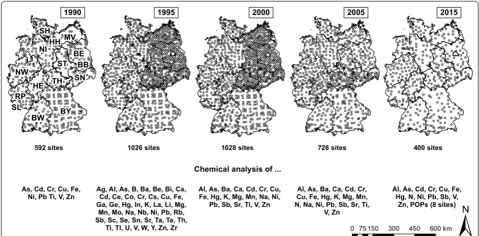
The number of sampling sites in six EMS between 1990 and 2015 ranged between 4499 and 7312 in 20 to 36 par-ticipating European countries. The number of sampling sites in five GMS (Fig. 1) was reduced from 1026 (1995) and 1028 (2000), respectively, to 726 (2005) and, further on, to 400 (2015) according to a transparent and statisti-cally sound methodology [34, 45, 46, 59]. In addition to Cd, Hg, Pb and N, aluminium (Al), arsenic (As), chro-mium (Cr), copper (Cu), nickel (Ni), vanadium (V) and zinc (Zn) were determined in the moss specimens col-lected in 2015. This article focus on the LRTAP elements Cd, Hg, Pb and N. Additionally, Cr is regarded, since this is one of the elements besides antimony (Sb) and Zn with an intermediate increase in concentration between 2000 and 2005.
This study aims at synoptically compare the spatial structures of element concentrations accumulated in moss in terms of surface maps as derived from sample point data by analysis and modelling of the spatial auto-correlation by means of Variogram analysis and, based on the resulting function, mapping by Kriging interpo-lation [24, 25]. Generalising spatial and temporal sam-ple data is an essential goal of empirical sciences. In BY
NI
BW
NW ST BB
HE MV
RP
SN TH SH
SL
BE HH
1990 1995 2000 2005 2015
592 sites 1026 sites 1028 sites 726 sites 400 sites
Chemical analysis of ...
As, Cd, Cr, Cu, Fe,
Ni, Pb Ti, V, Zn Ag, Al, As, B, Ba, Be, Bi, Ca,Cd, Ce, Co, Cr, Cs, Cu, Fe, Ga, Ge, Hg, In, K, La, Li, Mg, Mn, Mo, Na, Nb, Ni, Pb, Rb, Sb, Sc, Se, Sn, Sr, Ta, Te, Th,
Ti, Tl, U, V, W, Y, Zn, Zr
Al, As, Ba, Ca, Cd, Cr, Cu, Fe, Hg, K, Mg, Mn, Na, Ni,
Pb, Sb, Sr, Ti, V, Zn
Al, As, Ba, Ca, Cd, Cr, Cu, Fe, Hg, K, Mg, Mn, N, Na, Ni, Pb, Sb, Sr, Ti,
V, Zn
Al, As, Cd, Cr, Cu, Fe, Hg, N, Ni, Pb, Sb, V,
Zn, POPs (8 sites)
0 75150 300 450 600km
Fig. 1 Sampling sites and elements regarded the German Moss Surveys (GMS) 1990, 1995, 2000, 2005, 2015. SH Schleswig-Holstein, MV
Mecklenburg-Western Pomerania, HH Hamburg, NI Lower Saxony, BE Berlin; ST Saxony-Anhalt, BB Brandenburg, NW North Rhine-Westphalia, SN
particular, spatial generalisation through interpolation is a precondition for connecting and evaluating measure-ments derived from monitoring networks being incon-gruent with the moss monitoring network [32–36]. The explanation of the course of investigation starts with the sampling procedure followed by the chemical analy-sis of element concentrations including quality control (QC; “Determination of element concentrations in moss” section). QC is an essential precondition for interpret-ing measurement differences at several points in space and time as real phenomena but not as artefacts. Then, descriptive statistics (“Descriptive statistics” section) and spatial statistics in terms of Moran’s I, Variogram analy-sis and Kriging interpolation (“Geostatistics” section) are outlined.
Methods
Determination of element concentrations in moss
The European moss surveys follow a harmonised meth-odology encompassing the design of the monitoring net-work, sampling and chemical analyses including QC and data handling. For EMS 2015, this was published by ICP Vegetation [16]. The fundamentals rely on Rühling et al. [48]. They were up-dated continuously [13] and, respec-tively, specified as, e.g., for Germany [62].
Regarding the reorganisation of the German sampling network, Nickel and Schröder [34] operationalised the given criteria of ICP Vegetation [16]. Examples include: The monitoring network should comprise 1.5 sampling sites within 1000 km2 or at least two sites per
EMEP-deposition modelling grid (50 km × 50 km), regions with steep deposition gradients should be sampled at a higher sample point density, moss sampling points should be located close to sites where atmospheric deposition is collected by technical devices, for enabling time trend analyses, the sampling points should remain the same across time, the sampling should be restricted to the three moss species mentioned in “Background” section.
After a thorough common training, the moss speci-mens were sampled from June 2016 until March 2017 by five experts according to ICP Vegetation [16]. The same is true for the preparation of the moss specimens by another five members of the lab staff which was subjected to continuous QC, too. The mass concentration of total N was performed according to VDLUFA [69] using an Elementar Vario Max. The dry and homogeneous moss material was digested with nitric acid (65%) and hydro-gen peroxide (35%) in a microwave Mars 5. The measure-ments of Al, As, Cd, Cr, Cu, Fe, Ni, Pb, Sb, V and Zn were performed according to ISO [18] using ICP-MS (Agilent 7900 with sample loop). Hg was determined according to
ISO [17] by cold vapour atomic absorption spectroscopy (AAS, Mercury) after enrichment with tin(II) chloride.
The limits of quantification for the elements were determined, and the respective results are given in “
Qual-ity control of measurement” section. The same applies
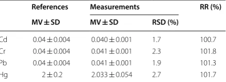
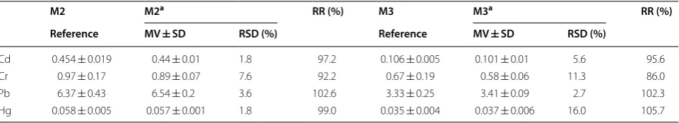
for the lab-internal QC encompassing for each sampling series the measurement of a blind value and of reference materials to check for recovery and performance. The moss reference materials M2 and M3 ([66] for recom-mended HM values; [12] for recommended HM and N values) were analysed together with three samples from the EMS 2005 (samples 2071, 3050, 3069) each three times. Lab-external QC was accomplished through certi-fication according to [19] and through national and inter-national ring tests.
Descriptive statistics
For ensuring the comparability of the five GMS, the same descriptive statistical parameters of GMS 2015 were used for all monitoring campaigns [14, 41, 53, 65]. Thus, for each trace element and N, mentioned in “Determination
of element concentrations in moss” section, minimum,
maximum, arithmetic mean, standards deviation, coef-ficient of variation in [%], the 20th, 50th, 90th and 98th percentiles were calculated by taking in consideration all sample point data and specifically for moss species and federal states [38]. In addition, the geostatistical surface estimations were also done (“Geostatistics” section) [62].
Geostatistics
Kriging interpolation. The semivariance reached at the maximum spatial extent of autocorrelation is called sill. The nugget-to-sill ratio [%] is a measure for the strength of spatial autocorrelation: The higher the ratio, the lower the autocorrelation. As a rule of thumb, the nugget-to-sill ratio should not exceed 75%. Ratio values nearby 100% indicate a random distribution of measurements [10, 22,
71].
A complementary statistical means to account for spa-tial autocorrelation is suggested by Moran [27]. Moran’s I allows for testing whether objects are spatially distrib-uted at random (negative I-values) or clustered (positive I-values) and whether spatial autocorrelation is signifi-cant. The range determined by Variogram analysis can be used in Moran’s I statistics to specify the spatial extent of autocorrelation [70].
Following the autocorrelation analysis and modelling, the autocorrelation function was used for Kriging inter-polation. Depending from assumptions about the random function, several variants of Kriging interpolation can be applied: two of them are ordinary Kriging, supposing the mean of the random function as constant across the area investigated, and Universal Kriging for data including a deterministic trend [22]. Since most data from environ-mental surveys do not follow a normal distribution [47], the moss survey data distribution was analysed with regard to their skewness (Sk), and data not normally dis-tributed were subjected to log-transformation [64] and Box-Cox-transformation [49, 71]. The quality of Krig-ing interpolation was quantified by leave-one-out cross-validation [15, 22]. Thereby, the mean error (ME) and the mean standardized error (MSE) indicate over- and underestimation. Optimal values of both measures would be 0. The root mean square standardised error (RMSSE) accounts for the relation between theoretical and experi-mental variance. Its optimum value is 1, and RMSSE < 1 indicates underestimation and RMSSE > overestimation. The median of percentage errors (MPE [%]) allows for comparing data covering different orders of magnitude. Cases where cross-validation measures show smaller ranges than empiric measurements indicate a good qual-ity of spatial estimation. To account for this, the cor-rected mean percentage error (MPEc) can be computed by multiplying MPE with the ratio of the empirical and estimated ranges. Additionally, Olea [40] suggests the correlation coefficient r (Pearson) between estimated and empiric measurements which ideally equal 1.
The geostatistical analyses and modelling were com-puted by ESRI ArcGIS 10.2‚ Geostatistical Analyst. For ensuring the reproducibility of spatial estimation, the primary data and all statistical measures explained above were documented and archived [62].
Results
Quality control of measurement
The limits of quantitative detection of elements in moss specimens (Table 1) are within the ranges of the refer-ence materials indicated in Tables 2, 3, 4. Similar results are shown in the quality control for Al, As, Cu, Fe, Ni, Sb, V and Zn (Additional file 1: Tables S1–S3).
The element concentrations for M2 and M3 meas-ured in this research did not differ significantly from the respective reference values (RR% < 10%), with the excep-tion of Cr (14%, M3). This means that the recovery rate mainly was above 90% (Table 4). All measurements of elements concentrations in M2 and M3 with the excep-tion of Zn (M2) were within the ranges published by Har-mens et al. [12] and Steinnes et al. [66] (Table 4).
Table 1 Limits of quantification (LQ) for the elements determined
a In mg/kg (HM) and mass-% (N)
Cd Cr Pb Hg N
LQa 0.05 0.05 1.00 0.020 0.01
Table 2 Statistical values for determination of nitrogen in reference materials during the measurement period
MV ± SD mean value ± standard deviation (in mg/kg), RSD relative standard deviation, RR recovery rate, related to the reference, TBK6 Kinesin-like polypeptides 6
References Measurements RR (%)
MV ± SD MV ± SD RSD (%)
Carbamide 46.62 ± 2.33 47.05 ± 0.81 1.7 100.9 Glutamic acid 9.52 ± 0.95 9.58 ± 0.18 1.9 100.7 TBK6 0.156 ± 0.01 0.16 ± 0.01 5.8 103.5
Table 3 Statistical values for determinations of heavy metals in reference materials during the measurement period
MV ± SD mean value ± standard deviation (in mg/L, µg/L for Hg), RSD relative standard deviation, RR recovery rate, related to the reference
References Measurements RR (%)
MV ± SD MV ± SD RSD (%)
Geostatistically analysed, modelled and mapped spatial structures of element concentrations in moss 1990–2015
The presentation of results of geostatistical analysis, modelling and mapping explained in “Descriptive statis-tics” section focus on those elements relevant for CLR-TAP, i.e. Cd, Hg, Pb and N and on Cr representing those three elements which did not show a continuous decrease between 1990 and 2015 but an intermediate increase from 2000 to 2005 (Cr, Sb, Zn). Thereby, the results derived from the moss sampling 2015 are compared to those from previous campaigns. In addition, geostatisti-cal surface estimations of Al, As, Cu, Fe, Ni, Sb, V and Zn concentrations in moss and respective statistical values are provided in the supplement (Additional file 1: Fig-ures S1–S4; Tables S4 and S5).
Cadmium
The GMS 2015 yielded 398 Cd measurement values which were analysed by application of statistical meth-ods explained in “Methods” section. With values between 0.035 and 1.760 mg/kg Plesch shows lower 20th, 50th, 90th and 98th percentiles than Hypcup and Psepur [62]. Regarding the federal states, Cd concentrations in North Rhine-Westphalia show the highest median value (0.189 mg/kg). The Cd median of the federal states Hesse, Mecklenburg-Western Pomerania, Saarland, Sax-ony and Thuringia exceeds the Germany-wide median (= 0.136 mg/kg Cd). The lowest Cd median below the 20th percentile (= 0.0944 mg/kg) was found in Hamburg (= 0.089 mg/kg) [62].
Due to skewness (Sk = 6.28), Cd measurement values 2015 were transformed (Box Cox) before spatial gener-alisation by Universal Kriging. The spherical variogram model shows a low, but significant autocorrelation with a range of 223 km and a nugget-to-sill ratio of 0.66. Due to the high nugget effect, there is a considerable smoothing of the estimated values’ map. The results of cross-validation indicate a rather unbiased spa-tial estimation (MSE = − 0.07; RMSSE = 1.2) with low correlations between measurements and estimations
(rp = 0.22). The MPEc accounts for 12.55%. Figure 2
depicts increased Cd concentrations from North Rhine-Westphalia to Saxony. Further the maps show the trends of Cd accumulation in moss specimens col-lected between 1990 and 2015. During this period, the Germany-wide median of Cd concentrations decreased by 52.5%. Between 1990 and 1995 the median Cd accu-mulation in moss increased by + 2.1%, and from 1995 to 2005 it decreased by − 28.3%. No changes of the median Cd values throughout Germany could be meas-ured between 2000 and 2005, while from 2005 to 2015 the median Cd concentrations in moss decreased sig-nificantly by − 35.2%. Above-average decreased values were found between 2005 and 2015 in Baden-Wuert-temberg (− 35.8%), North Rhine-Westphalia (− 40%), Rhineland Palatinate (− 57.3%), Schleswig-Holstein (− 41.3%) and Saxony-Anhalt (− 37.4%). No increase of median Cd concentrations could be detected during the years 2005 to 2015 [38].
Chromium
The moss survey 2015 yielded Cr measurements from 399 sites with values ranging between 0.051 and 4.951 mg/kg. Hypcup exhibited higher 20th, 50th, 90th and 98th percentile values than Plesch and Psepur. Accordingly, the highest value in Germany (4.951 mg/ kg) was found in a Hypcup sample in Baden-Wuerttem-berg (BW450). Spatial clusters of values in this mag-nitude can be found in North Rhine-Westphalia (Ruhr Region), along the upper Rhine Valley (Baden-Wuert-temberg), in north and central Hesse, in Saxony-Anhalt and Saxony as well as in Bavaria, Lower Saxony and Saarland. The values in Brandenburg, Hesse, Hamburg, Lower Saxony, North Rhine-Westphalia, Rhineland Palatinate and Saarland are above the Germany-wide Cr median value (= 0.57 mg/kg). The lowest median Cr concentration was found in Mecklenburg-Western Pomerania (= 0.34 mg/kg).
The geostatistical surface estimation of Cr concentra-tions was performed by application of Ordinary Kriging. Table 4 Statistical values of the moss reference materials M2 and M3
MV ± SD mean value ± standard deviation (in mg/L, µg/L for Hg), RSD relative standard deviation, RR recovery rate, related to the reference a Measurements
M2 M2a RR (%) M3 M3a RR (%)
Reference MV ± SD RSD (%) Reference MV ± SD RSD (%)
Due to skewness (Sk = 3.17), the data were Box-Cox-transformed. An exponential model variogram was fit-ted to the empirical variogram indicating a low but significant (p < 0.01) spatial autocorrelation with a range of 104 km and a nugget/sill ratio of 0.67. The cross-vali-dation proved a low bias (MSE = − 0.01; RMSSE = 0.96), and the MPEc accounted for 20.38%.
Figure 3 presents the temporal and spatial develop-ment of Cr accumulation from 1990 to 2015. The maps corroborate a comprehensive decrease of Cr concentra-tions throughout Germany. From 2000 to 2005, the val-ues increased remarkably.
From 2000 to 2005, the Cr concentrations in moss increased. Hot spots can be found in the Ruhr Region (North Rhine-Westphalia), in the North-West of Lower Saxony, Saxony, Saxony-Anhalt and in Mecklenburg-Western Pomerania. From 2005 to 2015, the Cr accumu-lation in moss specimens decreased clearly.
The significant decrease of Cr median values between 1990 and 2000 accounted for 58.5% throughout Germany. However, from 2000 to 2005 the German Cr median increased by + 159.3% (p > 0.05). The highest rise was found in Mecklenburg-Western Pomerania (+ 754.5%). From 2005 and 2015, the reduction was 75.8% and between 1990 and 2015 it accounted for 74% [38].
Mercury
In 2015, 397 Hg measurements ranged between 0.0047 mg/kg and 0.1960 mg/kg. Regarding the 20th, 50th, 90th and 98th percentile values, there are no strik-ing differences between the moss species.
Since the Hg measurements were skewed (Sk = 3.33), they were Box-Cox-transformed, then interpolated by means of Ordinary Kriging, and finally back transformed. For the spherical autocorrelation function fitted to the experimental variogram autocorrelation is weak but could be proved to be statistically significant with a sill of 67 km and a nugget-to-sill ratio of 0.63. Cross-validation indicates a rather low bias (MSE = − 0.02; RMSSE = 1.37) with correlations of measurements and estimated values (rp = 0.33). The mean relative corrected deviance between
empiric measurements and geostatistically estimated val-ues is low (MPEc = 5.21%).
The Kriging maps in Fig. 4 depict the spatial and tem-poral trends of Hg bioaccumulation in moss due to atmospheric deposition between 1995 and 2015. The values are low in terms of the European classification of measurement values to be applied. From 1995 to 2000, slight increases can be proved in the Eastern part of Schleswig-Holstein, in the South of Saxony-Anhalt, Northern Thuringia, and in Baden-Wuerttemberg. Large-area Hg bioaccumulation occurred in North Rhine-Westphalia. During 2000 to 2005, further decline of Hg
concentrations in moss occurs throughout Germany. From 2005 to 2015, the Hg accumulation decreased in regions located in Bavaria, North Rhine-Westphalia, Sax-ony, Saxony-Anhalt, Mecklenburg-Western Pomerania. Contrary to that trend, increases of Hg concentrations could be localised in Lower Saxony. During 1990 to 2015, the Rhine valley in Baden-Wuerttemberg, Northern Thuringia, in the Erz Mountains (Saxony) and in Meck-lenburg-Western Pomerania are regions with continuous enhanced values.
In 2015, the 98th percentile of Hg concentrations in moss amounted to 0.0702 mg/kg, the 90th percentile to 0.054 mg/kg, and the median throughout Germany was 0.0446 mg/kg). The medians measured from 1995 to 2000 increased significantly in Baden-Wuerttemberg, Rhine-land Palatinate, Saxony-Anhalt and Thuringia. Across Germany, no such statistically significant trend could be corroborated. From 2000 to 2005, the median of Hg measurements sank in almost all federal states, and the median decreased by 14.6%, and during 2005 to 2015 the median values of Hg concentrations in moss accounted for another 4% (p < 0.05). Since 2005, the trends of Hg bioaccumulation were as follows: Increases could be proved for Brandenburg (+ 27.8%) and Lower Saxony, (+ 14.8%), while reductions were measured in Bavaria, (− 18.2%), North Westphalia (− 25.8%), Rhine-land Palatinate (− 5.7%) and Saxony (− 13.7%). The trend between 1995 and 2015 is characterised by a significant reduction throughout Germany by 20%, while spatial dif-ferences in terms of federal states range between − 51.2% (Bavaria) and + 17.4% (Brandenburg). Hesse, Hamburg, Lower Saxony, Rhineland Palatinate, Schleswig-Holstein, Saarland, Saxony-Anhalt and Thuringia did not show any significant decline since 1995 [38].
Lead
19 90 19 95 20 00 20 05 20 15 Cadm iu m Mo ni to ring si te Cd [m g/ kg ] >0 ,9 0, 8-0, 9 0, 7-0, 8 0, 6-0, 7 0, 5-0, 6 0, 4-0, 5 0, 3-0, 4 0, 2-0, 3 <0 ,2 Mo ni to ring si te Cd [m g/ kg ] >0 ,9 0, 8-0, 9 0, 7-0, 8 0, 6-0, 7 0, 5-0, 6 0, 4-0, 5 0, 3-0, 4 0, 2-0, 3 <0 ,2 Moni to ring si te Cd [m g/ kg ] >0 ,9 0, 8-0, 9 0, 7-0, 8 0, 6-0, 7 0, 5-0, 6 0, 4-0, 5 0, 3-0, 4 0, 2-0, 3 <0 ,2 Mo ni to ring si te Cd [m g/ kg ] >0 ,9 0, 8-0, 9 0, 7-0, 8 0, 6-0, 7 0, 5-0, 6 0, 4-0, 5 0, 3-0, 4 0, 2-0, 3 <0 ,2 Fig . 2 Spatial distr
ibution of sample point
-specific measur
ed and geostatistically estimat
ed C
19
90
19
95
20
00
20
05
20
15
Ch
ro
mium
Mo
ni
to
ring
si
te
s
Cr
[m
g/
kg
]
<8 7-8 6-7 5-6 4-5 3-4 2-3 1-2 <1
Mo
ni
to
ring
si
te
s
Cr
[m
g/
kg
]
<8
7-8
6-7
5-6
4-5
3-4
2-3
1-2
<1
Mo
ni
to
ring
si
te
s
Cr
[m
g/
kg
]
<8
7-8
6-7
5-6
4-5
3-4
2-3
1-2
<1
Mo
ni
to
ring
si
te
s
Cr
[m
g/
kg
]
<8
7-8
6-7
5-6
4-5
3-4
2-3
1-2
<1
Fig
. 3
Spatial distr
ibution of sample point
-specific measur
ed and geostatistically estimat
19
95
20
00
20
05
20
15
Me
rc
ur
y
Mo ni to ring si te Hg [m g/ kg ] >0 ,1 8 0, 16 -0 ,1 8 0, 14 -0 ,1 6 0, 12 -0 ,1 4 0, 1-0, 12 0, 08 -0 ,1 0, 06 -0 ,0 8 0, 04 -0 ,0 6 <0 ,0 4 Mo ni to ring si te Hg [m g/ kg ] >0 ,1 8 0, 16 -0 ,1 8 0, 14 -0 ,1 6 0, 12 -0 ,1 4 0, 1-0, 12 0, 08 -0 ,1 0, 06 -0 ,0 8 0, 04 -0 ,0 6 <0 ,0 4 Mo ni to ring si te Hg [m g/ kg ] >0 ,1 8 0, 16 -0 ,1 8 0, 14 -0 ,1 6 0, 12 -0 ,1 4 0, 1-0, 12 0, 08 -0 ,1 0, 06 -0 ,0 8 0, 04 -0 ,0 6 <0 ,0 4 Fig . 4 Spatial distribution of sample point
-specific measur
ed and geostatistically estimat
The decrease of Pb concentrations in moss trends col-lected in the federal states during 1990–2015 was statis-tically significant with the exception of Hamburg (n= 3) and ranged between − 81.3% (Schleswig-Holstein) and − 92.1% (Saxony) [38].
The spatial estimation and surface covering mapping of Pb bioaccumulation were calculated by Ordinary Kriging from Box-Cox-transformed data. The original measure-ment data were clearly skewed (Sk = 4.42). The expo-nential model variogram indicated a low but significant spatial autocorrelation with a range amounting to 202 km and a nugget-to-sill ratio of 0.70. The MSE (= − 0.04) proved a rather unbiased estimation and the RMSSE (= 1.24) points out an overestimation. The correlation between measurements and estimations was rp = 0.28
and the MPEc was 23.9%.
The Kriging map for the GMS 2015 (Fig. 5) is covered with estimated Pb concentrations < 5 mg/kg. Within this range, regions with estimation > 2.62 mg/kg are located in Hamburg and around (Schleswig-Holstein), in Lower Saxony (Harz mountains), in Saxony, in the Rhine valley (Baden-Wuerttemberg) and in North Rhine-Westphalia.
Figure 5 also depicts the spatial and temporal devel-opment of Pb concentrations from 1990 to 2015. The maps prove a Germany-wide continuous decrease of Pb bioaccumulation. The most distinct decline was proved for North Rhine-Westphalia, Brandenburg (Southern regions) and Saxony (Lausitz and Erz Mountains).
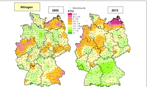
Nitrogen
From the measured concentrations of N in 400 moss specimens, ranging between 0.80 and 3.49%, a median value of 1.431% was computed. Regarding all descrip-tive statistical measures computed, Psepur evidenced the highest values. The highest N concentration was found in Mecklenburg-Western Pomerania. N measurements exceeding the 90th percentile (= 2.131%) could only be found in Mecklenburg-Western Pomerania, Schleswig-Holstein, Lower Saxony, North Rhine-Westphalia and Hesse. Ranking the German federal states by N concen-trations accumulated in moss, Mecklenburg-Western Pomerania shows the highest median value (= 2.370%), followed by North Rhine-Westphalia, Lower Saxony, Hesse, Thuringia, Schleswig-Holstein and Saxony, all exceeding the Germany-wide median N concentration in moss. The lowest median N values were found for Ham-burg and Saarland (1.190% and 1.115%, respectively).
The geostatistical estimation of surface covering N concentration in moss was performed by using second-order Universal Kriging of log-transformed measure-ment values. The spherical model variogram fitted to the experimental one corroborates a slight but signifi-cant spatial autocorrelation with a range of 117 km and
a nugget-to-sill ratio of 0.67. However, the estimation is nearly unbiased (MSE = − 0.03; RMSSE = 0.97) with low differences between measured and estimated values (MPEc = 2.96%) which are correlated with rp= 0.57.
Within the spatial patterns depicted in Fig. 6, the high-est surface high-estimations with values > 2.4% cover most of the territory of Mecklenburg-Western Pomerania. Esti-mations between 2.2 and 2.4% can be observed in Lower Saxony and North Rhine-Westphalia, especially in the western regions close to the border between both Ger-man federal states and the Netherlands. N concentra-tions > 1.6% cover wide areas of Schleswig-Holstein, Hesse, Thuringia and Saxony. N concentrations < 1.0% occur dominantly in the Alps.
The Kriging maps for 2005 and 2015 shown in Fig. 6
indicate that the N bioaccumulation did not change significantly during the last 10 years. However, this Germany-wide statistical statement includes regional decreases in Bavaria and Baden-Wuerttemberg and increases in Lower Saxony, Hamburg and in Mecklen-burg-Western Pomerania. Permanent N hot spots existed between 2005 and 2015 in North Rhine-Westphalia and Mecklenburg-Western Pomerania. Inference sta-tistical tests corroborate that the N concentrations did not change significant between 2005 and 2015 neither Germany-wide nor in most of the federal states. Sig-nificant increases were proved for Hamburg (− 33.1%), Mecklenburg-Western Pomerania (− 30.4%) and Bavaria (− 13.9%). Significant decreases of N concentrations in moss were determined for Baden-Wuerttemberg (− 13.9%).
Discussion
To evaluate the results presented, the discussion includes not only the elements presented in this article (Cd, Cr, Hg, Pb; N) but also some of those which could not be tackled. The spatial patterns of As, Cd, Ni, Pb, Sb and Zn detected in the GMS 2015 were rather similar to those mapped for the GMS 1995, 2000 and 2005. This similarity was quantified by means of Pearson correlation between the respective Kriging maps which accounted in case of As, Ni and Sb for rP > 0.4 (exceptions: As 2000, Sb 1995)
and in case of Cd, Pb and Zn for rp > 0.6. Continuous
19
90
19
95
20
00
20
05
20
15
Le
ad
Mo
ni
to
ring
si
te
Pb
[m
g/
kg
]
>4
0
35
-4
0
30
-3
5
25
-3
0
20
-2
5
15
-2
0
10
-1
5
5-10
<5
Mo
ni
to
ring
si
te
Pb
[m
g/
kg
]
>4
0
35
-4
0
30
-3
5
25
-3
0
20
-2
5
15
-2
0
10
-1
5
5-10
<5
Mo
ni
to
ring
si
te
Pb
[m
g/
kg
]
>4
0
35
-4
0
30
-3
5
25
-3
0
20
-2
5
15
-2
0
10
-1
5
5-10
<5
Mo
ni
to
ring
si
te
Pb
[m
g/
kg
]
>4
0
35
-4
0
30
-3
5
25
-3
0
20
-2
5
15
-2
0
10
-1
5
5-10
<5
Fig
. 5
Spatial distr
ibution of sample point
-specific measur
ed and geostatistically estimat
ed P
instance Pb, Sb), in the upper Rhine valley (mainly Al, As, Cr, Fe and Hg) and in Berlin (primarily Cr and Zn).
The development of bioaccumulation of heavy metals since 2005 is characterised by a Germany-wide signifi-cant decrease (p < 0.05). This general trend varies by ele-ment and region in terms of federal state. The range of decrease was between − 4% (Hg) to − 75.8% (Cr). Similar was the trend from the first measurement and 2015: The median values of heavy metals decreased significantly since 1990 and of Al, Hg and Sb since 1995. The most dis-tinct decrease was determined for Pb (− 85.9%), the low-est for Hg (− 20%). These trends of bioaccumulation are in agreement with the heavy metal emissions in Germany between 1990 and 2015 [30], especially in case of As, Cd, Ni and Pb. The concentrations of these four heavy metals in moss collected in 2005 on the one hand and modelled atmospheric deposition on the other hand were corre-lated with rS > 0.3 [38, 50, 51]. According to NaSE [30]
emissions from metallurgy (Cd, Ni and Pb), power econ-omy (As, Cd, Ni and Pb), manufacturing and construct-ing industry (As, Ni and Pb) and traffic (Pb) declined since 1990. However, the decrease of Hg bioaccumula-tion is less than the reducbioaccumula-tion of Hg emissions [30]. This is possibly due to long-range transport of gaseous Hg and atmospheric residence times of 6 to 18 months [52]. The concentrations of Cu and Zn in moss contradict the
emission trends. At least for Zn, the correlation between the concentration in moss ample in 2005 and the mod-elled atmospheric deposition is rs < 0.3 [38].
For Cr, good agreement could be identified between the emission trends [30] and the concentrations in moss during the period 1990 to 2015. Strikingly, the Cr con-centrations in moss were extraordinarily high in 2005, especially in Mecklenburg-Western Pomerania and con-urbations such as Bremen, Hamburg, Dresden, Halle/ Leipzig and the Ruhr region. Respective increased values were also reported from Austria and were attributed to a Cr mine on the Kola Peninsula [23, 38].
The spatial pattern of N concentrations in moss speci-mens collected in 2015 is in a more distinctive agree-ment than those determined in 2005 with what could be expected from the spatial patterns of potential emission sources: Regions with high spatial livestock density as for instance the Northwestern part of Lower Saxony and North Rhine-Westphalia show high N bioaccumulation and corroborate other investigations [26, 28, 29, 54]. The N emissions between 2005 and 2015 declined by 23.9% in case of NOx emissions. In 2015, agricultural land use
emitted 95% of the NH3 in Germany which increased
between 2005 and 2015 by 12% [31]. In conclusion, this should be evidenced by quantitatively correlating the spatial livestock density with the Kriging maps. Further, it
2005 2015
Nitrogen Monitoring site
N [%]
>2,4 2,2 - 2,4 2 - 2,2 1,8 - 2 1,6 - 1,8 1,4 - 1,6 1,2 - 1,4 1 - 1,2 <1
should be investigated whether the replacement of Plesch through the more nitrophilous Psepur could be a relevant influence.
Conclusions
The maps given in Figs. 2, 3, 4, 5, 6 are based on an inter-national classification [16] which does not allow detail-ing much regional variance due to decreasdetail-ing element concentrations in moss. Therefore, element- and cam-paign-specific percentile statistics should be computed ensuring to map the still existing spatial variance of ele-ment concentrations statistically sound. Based on this, heavy metals integrating Multi Metal Index should be computed and mapped according to Pesch and Schröder [42, 43, 44] and Schröder and Pesch [56–60] allowing to comprehend the many data collected from 1990 to 2015, to integrate several elements in one map depicting their spatial patterns according to their percentile statistics and not according to the international classification [16].
Additional file
Additional file 1: Table S1. Limits of quantification (LQ) for the elements
determined. Table S2. Statistical values for determinations of heavy
metals in reference materials during the measurement period. Table S3.
Statistical values of the moss reference materials M2 and M3. Table S4a.
Geostatistical analysis 2015: Methods and parameters of the model.
Table S4b. Geostatistical analysis 2015: Quality parameters of the model.
Figure S1. Spatial distribution of sample point-specific measured and
geostatistically estimated concentrations of Al and As in moss. Figure S2.
Spatial distribution of sample point-specific measured and geostatistically
estimated concentrations of Cu and Fe in moss. Figure S3. Spatial
distri-bution of sample point-specific measured and geostatistically estimated
concentrations of Ni and Sb in moss. Figure S4. Spatial distribution of
sample point-specific measured and geostatistically estimated
concentra-tions of V and Zn in moss. Table S5. Spatial distribution of sample
point-specific measured and geostatistically estimated V and Zn concentrations in moss.
Abbreviations
AAS: atomic absorption spectroscopy; Al: aluminium; As: arsenic; BB: Branden-burg; BE: Berlin; BW: Baden-Wuerttemberg; BY: Bavaria; Cd: cadmium; CLRTAP: convention on long-range transboundary air pollution; Cr: chromium; Cu: cop-per; CV: coefficient of variation; EMEP: European Monitoring and Evaluation Programme; EMS: European moss survey; Fe: iron; GMS: German moss surveys;
HE: Hesse; Hg: mercury; HH: Hamburg; HM: heavy metals; Hypcup: Hypnum
cupressiforme; ICP: International Cooperative Programme; ICP-MS: inductively coupled plasma–mass spectrometry; ISO: International Organization for Standardization; LQ: limit of quantification; M2, M3: moss reference materials; ME: mean error; MPE: median of percentage errors; MPEc: corrected mean percentage error; MSE: mean standardized error; MV: Mecklenburg-Western
Pomerania; MV: mean value; N: nitrogen; n: sample size; NH3: ammonia; NI:
lower Saxony; Ni: nickel; NOx: nitrogen oxide; NW: North Rhine-Westphalia;
p: level of significance; Pb: lead; Plesch: Pleurozium schreberi; POP: persistent
organic pollutants; Psepur: Pseudoscleropodium purum; QC: quality control;
RMSSE: root mean square standardised error; RP: Rhineland Palatinate; rp:
correlation coefficient (Pearson); RR: recovery rate; rs: correlation coefficient
(Spearman); RSD: relative standard deviation; Sb: antimony; SD: standard deviation; SH: Schleswig-Holstein; Sk: skewness; SL: Saarland; SN: saxony; ST:
Saxony-Anhalt; TBK6: kinesin-like polypeptides 6; TH: Thuringia; UNECE: United Nations Economic Commission for Europe; V: vanadium; Zn: zinc.
Acknowledgements
This research paper was only possible through the help and support of the Federal Environmental Agency, Dessau-Roßlau, Germany.
Authors’ contributions
WS headed the computations executed by SN. WS wrote the article. All authors read and approved the final manuscript.
Funding
Federal Environmental Agency, Dessau-Roßlau, Germany.
Availability of data and materials
The datasets generated and/or analysed during the current study are not publicly available due to copyright but are available from the corresponding author on reasonable request.
Ethics approval and consent to participate
Not applicable.
Consent for publication
Not applicable.
Competing interests
The authors declare that they have no competing interests.
Received: 27 March 2019 Accepted: 15 May 2019
References
1. Aas W, Breivik K (2009) Heavy metals and POP measurements 2007. EMEP/CCC-Report 3/2009. Norwegian Institute for Air Research, Kjeller,
Norway. https ://www.nilu.no/proje cts/ccc/repor ts/cccr3 -2009.pdf.
Accessed 31 Jan 2019
2. Balla S, Uhl R, Schlutow A, Lorentz H, Förster M, Becker C (2013) Untersu-chung und Bewertung von straßenverkehrsbedingten
Nährstoffeinträ-gen in empfindliche Biotope. https ://www.bast.de/BASt_2017/DE/Verke
hrste chnik /Publi katio nen/Downl oad-Publi katio nen/Downl oads/V-Naehr stoff eintr ag.pdf. Accessed 31 Jan 2019
3. Bill R (2010) Grundlagen der Geoinformationssysteme. 5., völlig neu bearbeitete Auflage. Wichmann Verlag, Heidelberg
4. Bobbink R, Hicks K, Galloway J, Spranger T, Alkemade R, Ashmore M, Bus-tamante M, Cinderby S, Davidson E, Dentener F, Emmett B, Erisman JW, Fenn M, Gilliam F, Nordin A, Pardo L, De Vries W (2010) Global assessment of nitrogen deposition effects on terrestrial plant diversity: a synthesis. Ecol Appl 20:30–59
5. Calmano W (2001) Untersuchung und Bewertung von Sedimenten: öko-toxikologische und chemische Testmethoden. Springer, Berlin Heidelberg 6. Colette A, Aas W, Banin L, Braban C F, Ferm M, González Ortiz A, Ilyin I,
Mar K, Pandolfi M, Putaud JP, Shatalov V, Solberg S, Spindler G, Tarasova O, Vana M, Adani M, Almodovar P, Berton E, Bessagnet B, Bohlin-Nizzetto P, Boruvkova J, Breivik K, Briganti G, Cappelletti A, Cuvelier K, Derwent R, D’Isidoro M, Fagerli H, Funk C, Garcia Vivanco M, Haeuber R, Hueglin C, Jenkins S, Kerr J, de Leeuw F, Lynch J, Manders A, Mircea M, Pay MT, Pritula D, Querol X, Raffort V, Reiss I, Roustan Y, Sauvage S, Scavo K, Simpson D, Smith RI, Tang YS, Theobald M, Tørseth K, Tsyro S, van Pul A, Vidic S, Wal-lasch M, Wind P (2016) EMEP Co-operative programme for monitoring and evaluation of the long-range transmission of air pollutants in Europe. Air pollution trends in the EMEP region between 1990 and 2012. Joint Report of EMEP Task Force on Measurements and Modelling (TFMM), Chemical Co-ordinating Centre (CCC), Meteorological Synthesizing Centre-East (MSC-E), Meteorological Synthesizing Centre-West (MSC-W).
EMEP/CCC-Report 1/2016. https ://www.unece .org/filea dmin/DAM/env/
docum ents/2016/AIR/Publi catio ns/Air_pollu tion_trend s_in_the_EMEP_ regio n.pdf. Accessed 31 Jan 2019
comparison to historical observations. Tellus B Chem Phys Meteorol 69:1–20
8. Frahm JP (1998) Moose als Bioindikatoren. Quelle & Meyer GmbH & Co, Wiesbaden
9. Fuchs S, Scherer U, Wander R, Behrendt H, Venohr M, Opitz D, Hillenbrand T, Marscheider-Weidemann F, Goetz T (2010) Berechnung von Stof-feinträgen in die Fließgewässer Deutschlands mit dem Modell MONERIS. Nährstoffe, Schwermetalle und Polyzyklische aromatische Kohlenwas-serstoffe. Texte – Umweltbundesamt, Dessau-Rosslau (Deutschland), 45/2010, 243 S
10. Goovaerts P (1999) Geostatistics in soil science: state-of-the-art and perspectives. Geoderma 89(1–2):1–45
11. Gruber JP (2001) Die Moosflora der Stadt Salzburg und ihr Wandel im Zeitraum von 130 Jahren. Stapfia 79:3–155
12. Harmens H, Norris DA, Steinnes E, Kubin E, Piispanen J, Alber R, Alek-siayenak Y, Blum O, Coşkun M, Dam M, De Temmerman L, Fernández JA, Frolova M, Frontasyeva M, González-Miqueo L, Grodzińska K, Jeran Z, Korzekwa S, Krmar M, Kvietkus K, Leblond S, Liiv S, Magnússon SH,
Maňkovská B, Pesch R, Rühling Å, Santamaria JM, Schröder W, Špirić Z,
Suchara I, Thöni L, Urumov V, Yurukova L, Zechmeister HG (2010) Mosses as biomonitors of atmospheric heavy metal deposition: spatial and temporal trends in Europe. Environ Pollut 158:3144–3156
13. Harmens H, Mills G, Hayes F, Sharps K, Frontasyeva M, the participants of the ICP Vegetation (2015) Air pollution and vegetation, annual report 2014/2015. ICP Vegetation Programme Coordination Centre, CEH Bangor, UK
14. Herpin U, Lieth H, Markert B (1995) Monitoring der Schwermetallbelas-tung in der Bundesrepublik Deutschland mit Hilfe von Moosanalysen. UBA-Texte 31/95
15. Isaaks EH, Srivatava RM (1989) An introduction to applied geostatsitics. Oxford University Press, New York
16. ICP Vegetation (2014) Monitoring of atmospheric deposition of heavy metals, nitrogen and POPs in Europe using bryophytes. Monitoring manual 2015 survey. United Nations Economic Commission for Europe Convention on Long-Range Transboundary Air Pollution. ICP Vegeta-tion Moss Survey CoordinaVegeta-tion Centre, Dubna, Russian FederaVegeta-tion, and Programme Coordination Centre. Bangor, Wales, UK
17. ISO (2005) DIN EN ISO 16772:2005-06, Bodenbeschaffenheit - Bestim-mung von Quecksilber in Königswasser-Extrakten von Boden durch Kaltdampf-Atomabsorptionsspektrometrie oder Kaltdampf-Atomflu-oreszenzspektrometrie (ISO 16772:2004), Ausgabe: 2005-06
18. ISO (2017) DIN EN ISO 17294-2:2017-01, Wasserbeschaffenheit - Anwend-ung der induktiv gekoppelten Plasma-Massenspektrometrie (ICP-MS) - Teil 2: Bestimmung von ausgewählten Elementen einschließlich Uran-Isotope (ISO 17294-2:2016); Deutsche Fassung EN ISO 17294-2:2016, Ausgabe: 2017-01
19. ISO/IEC (2005) DIN EN ISO/IEC 17025:2005-08, Allgemeine Anforder-ungen an die Kompetenz von Prüf- und Kalibrierlaboratorien (ISO/IEC 17025), Ausgabe: 2005-08
20. Jenssen M, Hofmann G, Nickel S, Pesch R, Riediger J, Schröder W (2013) Bewertungskonzept für die Gefährdung der Ökosystemintegrität durch die Wirkungen des Klimawandels, Kombination mit Stoffeinträgen unter Beachtung von Ökosystemfunktionen und -dienstleistungen. Umwelt-forschungsplan des Bundesministeriums für Umwelt, Naturschutz und Reaktorsicherheit. Forschungsvorhaben 3710 83 214, UBA-FB 001834. Dessau: Umweltbundesamt, UBA-Texte 87/2013. p 381
21. Jenssen M, Schröder W, Nickel S (2015) Typisierung von Wald- und Forstökosystemen als Grundlage zur Einstufung ihrer Integrität. Integrität von Wald- und Forstökosystemen unter dem Einfluss von Klimawandel und atmosphärischen Stickstoffeinträgen – Teil I. Naturschutz und Land-schaftsplanung 47:391–399
22. Johnston K, Ver Hoef JM, Krivouchko K, Lucas N (2001) Using ArcGIS geo-statistical analyst. Environmental Systems Research Institute, Redlands 23. Kratz W, Schröder W (2010) Wider die Vernunft – zum Ende eines
Pro-gramms effektiver Umweltdatenerhebung in Bund-Länder-Kooperation. Umweltwiss Schadst Forsch 22:80–83
24. Krige DG (1951) A statistical approach to some basic mine valuation problems on the Witwatersrand. J Chem Metallurg Mining Soc S Afr 6:119–139
25. Matheron G (1965) Les variables régionalisées et leur estimation. Masson, Paris
26. Meyer M (2017) Standortspezifisch differenzierte Erfassung atmos-phärischer Stickstoff- und Schwermetalleinträge mittels Moosen unter Berücksichtigung des Traufeffektes und ergänzende Untersuchungen zur Beziehung von Stickstoffeinträgen und Begleitvegetation. Diss. Univ.
Vechta. http://voado .uni-vecht a.de/handl e/21.11106 /75. Accessed 31 Jan
2019
27. Moran PAP (1950) Notes on continuous stochastic phenomena. Biom-etrika 37(1):17–23
28. Mohr K (1999) Passive Monitoring von Stickstoffeinträgen in Kiefern-forsten mit dem Rotstengelmoos (Pleurozium schreberi (Brid.) Mitt.). Umweltwiss Schadst Forsch 11:267–274
29. Mohr K (2007) Biomonitoring von Stickstoffimmissionen. Möglichkeiten und Grenzen von Bioindikationsverfahren. Umweltwissen-schaften und Schadstoff-Forschung 19:255–264
30. NaSE (2017) Nationale Trendtabellen für die deutsche Berichterstattung atmosphärischer Emissionen (Schwermetalle) 1990–2015, Stand Januar
2017, Umweltbundesamt, Dessau Roßlau. https ://www.umwel tbund
esamt .de/sites /defau lt/files /medie n/361/dokum ente/2018_02_14_em_ entwi cklun g_in_d_trend tabel le_hm_v1.0.xlsx. Accessed 31 Jan 2019 31. NaNE (2017) Nationale Trendtabellen für die deutsche Berichterstattung
atmosphärischer Emissionen (Stickstoff ) 1990–2015, Stand Januar 2017,
Umweltbundesamt, Dessau Roßlau. https ://www.umwel tbund esamt .de/
sites /defau lt/files /medie n/361/dokum ente/2018_02_14_em_entwi cklun g_in_d_trend tabel le_luft_v1.0.xlsx. Accessed 31 Jan 2019
32. Nickel S, Schröder W (2017) Integrative evaluation of data derived from biomonitoring and models indicating atmospheric deposition of heavy metals. Environ Sci Pollut Res 24:11919–11939
33. Nickel S, Schröder W (2017) Bestimmung von Schwermetalleinträgen in Waldgebiete mit Modellierung und Moosmonitoring. Schweizer Zeitschrift für Forstwesen 168(2):92–99
34. Nickel S, Schröder W (2017) Reorganisation of a long-term monitoring network using moss as biomonitor for atmospheric deposition in Ger-many. Ecol Ind 76:194–206
35. Nickel S, Schröder W (2017) Metalleinträge in terrestrische Ökosysteme: analyse von Daten aus Modellierung und Biomonitoring. Schweizerische Zeitschrift für Forstwesen 168(4):1–9
36. Nickel S, Schröder W, Fries C (2017) Synoptische Auswertung modellierter atmosphärischer Einträge von Schwermetallen und deren Indikation durch Biomonitore in Wäldern.Gefahrstoffe - Reinhaltung der Luft (Springer, VDI) 3/2017:75–90
37. Nickel S, Schröder W, Jenssen M (2015) Veränderungen deutscher Wälder durch Klimawandel und Stickstoffdeposition. Schweizerische Zeitschrift für Forstwesen 166(5):325–334
38. Nickel S, Schröder W (2018) Schwermetall- und Stickstoffkonzentrationen in Moosen deutscher Waldgebiete zwischen 1990 und 2015 - Ein Bund-Länder-Vergleich. Gefahrstoffe - Reinhaltung der Luft 78(3):95–108 39. Nultsch W (2012) Allgemeine Botanik, 12th edn. Thieme, Stuttgart 40. Olea RA (1999) Geostatistics for engineers and earth scientists. Kluwer
Academic Publishers, Boston
41. Pesch R, Schröder W, Genssler L, Goeritz A, Holy M, Kleppin L, Matter Y (2007) Moos-Monitoring 2005/2006: Schwermetalle IV und Gesa-mtstickstoff. Berlin (Umweltforschungsplan des Bundesministers für Umwelt, Naturschutz und Reaktorsicherheit. FuE-Vorhaben 205 64 200, Abschlussbericht, im Auftrag des Umweltbundesamtes), 90 S., 11 Tab., 2
Abb. (Texteil), 51 S. + 41 Karten, 34 Tabellen, 46 Diagramme (Anhang)
42. Pesch R, Schröder W (2006a) Mosses as bioindicators for metal accumula-tion: statistical aggregation of measurement data to exposure indices. Ecol Ind 6:137–152
43. Pesch R, Schröder W (2006b) Integrative exposure assessment through classification and regression trees on bioaccumulation of metals, related sampling site characteristics and ecoregions. Ecol Inf 1(1):55–65 44. Pesch R, Schröder W (2006c) Assessment of metal accumulation in
mosses by combining metadata, statistics and GIS. Nova Hed-wigia 82(3–4):447–466
45. Pesch R, Schröder W, Dieffenbach-Fries H, Genßler L (2007) Optimierung des Moosmonitoring-Messnetzes in Deutschland. Umweltwiss Schadst Forsch 20:49–61
47. Reimann C, Filzmoser P (2000) Normal and lognormal data distribu-tion in geochemistry: death of a myth. Consequences for the statisti-cal treatment of geochemistatisti-cal and environmental data. Environ Geol 39(9):1001–1014
48. Rühling A, Rasmussen L, Mäkinen A, Pilegaard K, Steinnes E, Nihlgard B (1989) Survey of the of the heavy-metal deposition in Europe using bryophytes as bioindicators: proposal for an international programme. Steering Body of Environmental Monitoring in the Nordic Countries 49. Sachs L, Hedderich J (2009) Angewandte Statistik. Methodensammlung
mit R. Springer, Berlin
50. Schaap M, Roemer M, Sauter F, Boersen G, Timmermans R, Builjes PJH, Vermeulen AT (2005) LOTOS-EUROS: Documentation, TNO report B&O-A R 2005/297
51. Schaap M, Timmermans RMA, Roemer M, Boersen GAC, Builtjes PJH, Sau-ter FJ, Velders GJM, Beck JP (2008) The LOTOS–EUROS model: description, validation and latest developments. Int J Environ Pollut 32(2):270–290 52. Schaap M, Hendriks C, Jonkers S, Builtjes P (2017) Impacts of heavy metal
emission on air quality and ecosystems across germany. Sources, trans-port, deposition and potential Hazards. part 1: assessment of the atmos-pheric heavy metal deposition to terrestrial ecosystems in Germany. Final
report FKZ3713 63 253. Dessau-Roßlau, Germany. https ://www.umwel
tbund esamt .de/sites /defau lt/files /medie n/1410/publi katio nen/2018-12-13_texte _106-2018_schwe rmeta llemi ssion en_en.pdf. Accessed 21 May 2019
53. Schröder W, Anhelm P, Bau H, Broecker F, Matter Y, Mitze R, Mohr K, Peiter A, Peronne T, Pesch R, Roostai AH, Roostai Z, Schmidt G, Siewers U (2002) Untersuchung von Schadstoffeinträgen anhand von Bioindikatoren. Aus- und Bewertung der Ergebnisse aus dem Moosmonitoring 1990, 1995 und 2000. Umweltforschungsplan des Bundesministers für Umwelt, Naturschutz und Reaktorsicherheit. FuE-Vorhaben 200 64 218, Abschluss-bericht Band 1, im Auftrag des Umweltbundesamtes, Berlin. 221 S., 29 Tab., 94 Abb
54. Schröder W, Hornsmann I, Pesch R, Schmidt G, Fränzle S, Wünschmann S, Heidenreich H, Markert B (2006) Stickstoff- und Metallakkumulation in Moosen zweier Regionen Mitteleuropas als Spiegel ihrer Landnut-zung? Umweltwissenschaften und Schadstoff-Forschung (Online First 24.11.2006), S. 1–12
55. Schröder W, Nickel S, Jenssen M, Riediger J (2015) Methodology to assess and map the potential development of forest ecosystems exposed to climate change and atmospheric nitrogen deposition: a pilot study in Germany. Sci Total Environ 521–522:108–122
56. Schröder W, Pesch R (2004a) The 1990, 1995 and 2000 moss monitoring data in Germany and other European countries. Trends and statistical aggregation of metal accumulation indicators. Gate to Environmental and Health Sciences, June 2004, pp. 1–25
57. Schröder W, Pesch R (2004b) Metal accumulation in mosses. Spatial analysis and indicator building by means of GIS, geostatistics and cluster techniques. Environ Monit Assess 98(1-3):131–156
58. Schröder W, Pesch R (2004c) Spatial and temporal trends of metal accu-mulation in mosses. J Atmos Chem 49:23–38
59. Schröder W, Pesch R (2005b) Geographische Umweltmessnetzanalyse und -planung. Geog Helv 60(2):77–86
60. Schröder W, Pesch R (2007) Synthesizing bioaccumulation data from the German metals in mosses surveys and relating them to ecoregions. Sci Total Environ 374:311–327
61. Schröder W, Nickel S, Schönrock S, Meyer M, Wosniok W, Harmens H, Frontasyeva MV, Alber R, Aleksiayenak J, Barandovski L, Danielsson H, de Temmermann L, Fernández Escribano A, Godzik B, Jeran Z, Pihl Karlsson G, Lazo P, Leblond S, Lindroos AJ, Liiv S, Magnússon SH, Mankovska B, Martínez-Abaigar J, Piispanen J, Poikolainen J, Popescu IV, Qarri F,
Santam-aria JM, Skudnik M, Špirić Z, Stafilov T, Steinnes E, Stihi C, Thöni L, Uggerud
HT, Zechmeister HG (2016) Spatially valid data of atmospheric deposition of heavy metals and nitrogen derived by moss surveys for pollution risk assessments of ecosystems. Environ Sci Pollut Res 23:10457–10476 62. Schröder W, Nickel S, Völksen B, Dreyer A (2018) Nutzung von
Bioindi-kationsmethoden zur Bestimmung und Regionalisierung von Schad-stoffeinträgen für eine Abschätzung des atmosphärischen Beitrags zu aktuellen Belastungen von Ökosystemen. F&E-Vorhaben 3715 63 212 0, Abschlussbericht, im Auftrag des Umweltbundesamtes, Dessau. Text 188
S. + 10 Anhänge (zusammen 376 S.)
63. Schröder W, Riediger J, Nickel S, Jenssen M (2016) Projektion zukünftiger Ökosystemzustände unter dem Einfluss von Klimawandel und atmos-phärischen Stickstoffeinträgen. Integrität von Wald- und Forstökosyste-men unter dem Einfluss von Klimawandel und atmosphärischen Stickst-offeinträgen – Teil II. Naturschutz und Landschaftsplanung 48(1):22–28 64. Shapiro SS, Wilk MB (1965) An analysis of variance test for normality
(complete samples). Biometrika 52:591–611
65. Siewers U, Herpin U (1998) Schwermetalleinträge in Deutschland. Moos-Monitoring 1995. Geologisches Jahrbuch, Sonderhefte, Heft SD 2, Bornträger, Stuttgart
66. Steinnes E, Rühling A, Lippo H, Mäkinen A (1997) A reference materials for large-scale metal deposition surveys. Accred Qual Assur 2:243–249 67. Travnikov O, Ilyin I (2005) Regional model MSCE-HM of heavy metal
trans-boundary air pollution in Europe. EMEP/MSC-E Technical Report 6/2005. p 59
68. Travnikov O, Ilyin I, Rozovskaya O, Varygina M, Aas W (2015) Heavy metals: analysis of long-term trends, country-specific research and progress in mercury regional and global modelling Meteorological Synthesizing Centre, East, Moscow (MSC-E, Russia) and Norwegian Institute for Air Research, Kjeller (CCC, Norway). MSC-E & CCC-Status Report 2/2015. p 70 69. VDLUFA (Verband Deutscher Landwirtschaftlicher Untersuchungs- und
Forschungsanstalten) (1995) Methodenbuch, Band II.1. Die Untersuchung von Düngemitteln, 3.5.2.7 Bestimmung von Gesamt-Stickstoff, Verbren-nungsmethode, 4. Aufl., Gesamtwerk einschl. 1.-6. Ergänzung (einschl. Ringordner), VDLUFA-Verlag, Darmstadt
70. Warf B (ed) (2010) Encyclopedia of geography. Sage Publications, Thou-sand Oaks
71. Webster R, Oliver MA (2001) Geostatistics for environmental scientists. Wiley, Chichester
72. WGE (2004) Review and assessment of air pollution effects and their recorded trends. Working group on effects, convention on long-range transboundary air pollution. National Environment Council UK
Publisher’s Note