Int. J. Data Envelopment Analysis (ISSN 2345-458X)
Vol.7, No.1, Year 2019 Article ID IJDEA-00422, 24 pages Research Article
A Novel Efficiency Ranking Approach Based
on Goal Programming and Data Envelopment
Analysis for the Evaluation of Iranian Banks
M. Nouri1, E. Mohammadi*2, M. Rahmanipour3
(1)
MSc in Industrial Engineering, Department of Industrial Engineering, University of Science and Technology, Tehran, Iran
(2)
Assistant Professor, Department of Industrial Engineering, University of Science and Technology, Tehran, Iran
(3)
MSc in Economics, Department of Progress Engineering, University of Science and Technology, Tehran, Iran
Received 23 July 2018, Accepted 14 December 2018
Abstract
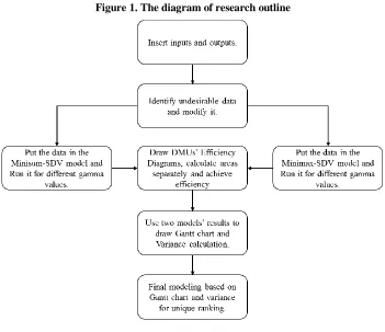
In the Iranian economy, banks play a key role in financing and developing the capital market. Therefore, it is important to evaluate the performance of stock banks. Data Envelopment Analysis (DEA) is a wide range of mathematical models used to measure the relative efficiency for a set of homogeneous decision-making units with similar inputs and outputs. In this paper, a novel efficiency ranking approach is proposed with two flexible mixed models derived from Goal Programming Data Envelopment Analysis (GPDEA) models. To solve this mismatch, we use Gantt chart to show DMUs’ floating ranking and use another model to appoint the ranks exactly. In this paper, we analyze 18 stocks efficiency from bank industry of Tehran Exchange in 2016 using the GPDEA approach. Results demonstrate that the novel efficiency ranking approach has higher ability than the basic models in efficiency ranking.
Keywords: bank, Data Envelopment Analysis, efficiency, Goal Programming.
*. Corresponding author: Email: [email protected]
1. Introduction
Financial institutions play a very important role in allocating resources, economic growth and job creation. For each country, the existence of financially viable companies is necessary to promote and support economic growth. Also, the banking is one of the most complex industries in the world and has a major share in the property and wealth of countries. In today's world, most banks are operating in a competitive and dynamic environment in which variables are constantly changing and it is difficult to predict these changes. On the other hand, banks spend a lot of time and money to achieve their goals.
To overcome this competitive
environment, many bank officials and academic researchers have tried to find ways to improve the performance of banks. With increasing the foreign and domestic competition and the provision of diverse banking services and products, there is a serious need to improve the performance of the branches to stay competitive. Therefore, the durability of banks in a new competitive environment requires the existence of efficient branches’ network. Due to the importance of this issue, the efficiency of active banks’ branches in Iran has been measured and investigated. Data Envelopment Analysis (DEA) is a non-parametric method, can be solved by linear programming, and is nowadays widely used in most countries to evaluate the systems’ performance with various activities such as maintaining airline bases, the police forces, banks, universities, insurance companies. In 1990, Aly et al. present a non-parametric frontier approach to calculate the total, technical, pure technical, allocative, and scale efficiencies for a sample of 322 independent banks. The sample was drawn from the Federal Deposit Insurance Corporation tapes on the Reports of Condition and Reports of Income (Call Reports) for the year
1986.The main source of efficiency was technical in nature, rather than allocative and the results showed a low level of overall efficiency. Separate efficiency frontiers were constructed to test the effect of branching, however, the distributions of efficiency measures for branching and non-branching banks were not found to be different [1]. Miller and Noulas considered the relative technical efficiency of 201 large banks from 1984 to 1990 using DEA. In their study, averages of bank technical inefficiency were just over 5 percent, much lower than that was found in existing estimates and larger and more profitable banks have higher levels of technical efficiency [2]. Wheelock and Wilson reviewed the technical advances, inefficiencies and productivity changes in banking from 1984 to 1993. He used three inputs and five outputs. His main findings are that commercial banks experience reduced productivity, and they are technically more inefficient from 1984 to 1993 [3]. Bal and Orkcu have solved a multi-criteria data envelopment analysis (MCDEA) model, used in the literature to moderate the homogeneity of weights dispersion, using pre-emptive GP. The MCDEA model is solved using pre-emptive GP gives the same relative efficiency as the classical DEA model while it improves the homogeneity of input-output weights. This conclusion is confirmed by the computational results obtained when the two models are applied to a real data set relative to the socio-economic performances of European countries and their randomly generated instances with different numbers of decision making units, inputs and outputs [4].
59
found a significant relationship between risk and efficiency [5]. Holod and Lewis proposed an alternative DEA model for bank efficiency that treats deposits as an intermediate product, thus emphasizing the dual role of deposits in the bank production process. Consequently, the amount of deposits’ effect on bank efficiency depends on the efficiency at both stages of the bank production process. The main advantage of their model was that it does not require a researcher to make a judgment call as to whether having more (production approach) or less (intermediation approach) deposits is ‘‘better’’ for bank efficiency. Their unified framework has the potential to produce more consistent efficiency estimates [6]. Halkos and Tzeremes have proposed a bootstrapped DEA-based procedure to pre-calculate and pre-evaluate the short-run operating efficiency gains of a potential bank merger or acquisition (M&A). They applied their proposed procedure to investigate the degree of operating efficiency gains of 45 possible bank M&As in the Greek banking over the period from 2007 to 2011 [7]. Bal et al. have developed two new models based on a multi-criteria data envelopment analysis (MCDEA) to moderate the homogeneity of weights distribution by using GP. These goal programming data envelopment analysis models, GPDEA-CCR and
GPDEA-BCC, also improve the
discrimination power of DEA [8].
Puri and Yadav have endeavored to propose a DEA model with undesirable outputs and further to extend it in fuzzy environment in view of the fact that input/output data are not always available in exact form in real life problems. They have proposed a fuzzy DEA model with undesirable fuzzy outputs which can be solved as a crisp linear program for (0, 1] using a-cut approach. Moreover, they have presented a numerical illustration followed
by an application to the banking sector in India using fuzzy input/output data for the period 2009–2011 [9]. Tsolas and Giokas evaluated the efficiency of the branches of a large Greek bank using two GP and DEA methods. They use a minimal absolute deviation (a special case of GP / limited regression) and DEA as two performance measurement methods. Performance evaluation using GP is examined using two conceptual alternative models: one focusing on the transaction, and the other on the efficiency of production. The DEA evaluation has been done using the productivity model under a constant and variable return rate. The results confirm a very strong relationship between the GP and DEA rankings [10]. Moghadam et al. have sought to study and investigate about two methods for measuring efficiency: DEA and GP. The result of this study is an integrate DEA and the GP model is designed to find out the bank performance’s weaknesses and alert the managers [11].
al. provide an integrated model of DEA and GP to improve the resolution, efficiency, and distribution of balanced and homogeneous weights by means of
corrective models (GPDEA-CCR,
GPDEA-BCC), and they provide the benefits of each of these corrective models with examples [13]. (Figure 1)
In this paper, we present a novel efficiency ranking approach. The proposed approach has two new flexible mixed models from three DEA basic models. The DEA basic models are based on Goal Programming. In order to Integration two models’ results, first we draw DMUs’ diagrams using multiple efficiencies, then calculate the graphs’ area to achieve efficiency. But each proposed models give us unique efficiency which are not the same. To solve the mismatch problems, we use
Gantt chart to show DMUs’ floating ranking and use another model to appoint the ranks exactly.
In the next section, the theoretical framework is presented. The novel approach’s mathematical modeling is introduced in Section 3. The information related to Iran's Banks is used for the proposed approach. In the fifth section, the results of this research have been studied.
2. Description of the theoretical framework
In this section, the theoretical framework for data envelopment analysis will be exhibited. First, the basic model of DEA is presented and then it is referred to due to the use of GP. Then, the basic DEA models based on GP are presented.
61 2.1. Data Envelopment Analysis
Data envelopment analysis (DEA) is a technique for measuring the relative efficiencies of decision making units (DMUs), using similar inputs to produce similar outputs where the multiple inputs and outputs are incommensurate in nature. DEA has been one of the fastest growing areas of Operations Research and Management Science in the past decade. DEA has been applied to a wide variety of managerial and economic problem situations in both the public and private sectors [14].
The DEA model for evaluating the efficiency of a DMU established by Charnes et al. [15] is as follows:
Max 0 0 1 s r r r
h u y
s.t. (І) 0 1 1, m i i i v x
1 1 0 s mr rj i ij
r i
u y v x
j 1,..., ,n, 0,
r i
u v for all r and i,
where j is the DMU index, j 1,...,n , r the output index, r 1,...,s , i the input
index, i 1,...,m,
y
ri the value of theoutput r for the DMU j,
x
ijthe value of theinput i for the DMU j,
u
rthe weight given to the output r,v
ithe weight given to the input i, andh
0 is the relative efficiency of unit under investigation, the DMU under evaluation. In this model, the unit under investigation is efficient if and only if0
1
h
. There are many different DEA models. Most frequently to deal with the problems of discriminating power and weight restriction Model (І) is proposed. We will develop our proposed model based on model (І). There are some othermultiple criteria approaches to DEA problems that are formulated based on different DEA models [16]. However, the focuses of those studies are somewhat different from ours.
Model (І) can be expressed equivalently in the following deviation variable form:
Min 0 0 1 1 s r r r
d u y
(П)s.t. 0 1 1 m i i i v x
1 1 0 s mr rj i ij
r i
u y v x
j 1,..., ,n, 0,
r i
u v for all r and i,
Where d0 is the deviation variable for unit
under investigation and dj the deviation
variable for the DMU j (appeared at the original inequality constraint j) in the model, the under investigation unit is efficient if and only if d00 or,
equivalently, h01.If the unit under
investigation is not efficient, its efficiency score is h0 1 d0.
2.2. DEA and Goal Programming
differentiate and present (s) the actual weights as follows.
2.2.1. Minimizing diversion variable model
Model (П) could be presented as an ideal planning model as follows:
Min
d
0 (a)s.t: 0 1 1 m i i i v x
1 1 0 s mr rj i ij j
r i
u y v x d
j1,...,n, 0
r i
u v for all r and i, Where
d
0 is the deviant variable for unitunder investigation and
d
j is thedeviating variable for unit j. The value of
0
d
in the range [0,1) represents theInefficiency value, the lower
d
0, the inefficiency is less for a unit (and therefore more efficient), so it can be said that this classical model seeks to minimize inefficiency of the unit under investigation that is measured withd
0 [17].2.2.2. Minimizing the total deviant variables model
Another method of Inefficiency measurement is a model that minimizes the total deviant variables. This model is called Minisum, and the general form of this model is as follows [18]:
Min 1 n j j d
(b)s.t: 0 1 1 m i i i v x
1 1 0 s mr rj i ij j
r i
u y v x d
j1,...,n, , 0
r i j
u v d for all r, i
and j
2.2.3. Minimizing the maximum deviation model
If the maximum deviation value is indicated by M, its related mathematical
relation can be written as
( 1,..., )
j
d M j n . Now, if M is smaller
and smaller, it means that the amount of deviations from the aspiration decreases. This model is called Minimax and is defined as follows [19]:
Min M (c)
s.t. 0 1 1 m i i i v x
1 1 0 s mr rj i ij j
r i
u y v x d
j1,...,n0
j
M d j 1,...,n
, , 0
r i j
u v d for all r, i
and j
2.3. Desirable or Undesirable Data
The general attitude in evaluating the efficiency of a unit is that reducing inputs and increasing outputs will improve performance. The CCR model is based on this attitude. However, it should be noted that organizations are not always seeking to maximize outputs and eliminate inputs because outputs and inputs can be desirable (good) or undesirable (bad). Another method is reducing unpredictable data in the model. If 𝑦𝑟𝑗𝑔 represents the desirable output (good) and 𝑦𝑟𝑗𝑏 represents
the undesirable (bad) output, we want to increase 𝑦𝑟𝑗𝑔 and decrease 𝑦𝑟𝑗𝑏 to improve performance. Nevertheless, in multi-axis input-output models with constant output, both outputs 𝑦𝑟𝑗𝑏 and 𝑦𝑟𝑗
𝑔
are increased to improve performance. Here, to increase the desirable output and reduce undesired output, we first multiply the undesired outputs in (-1), and then add the value of 𝑡𝑟 to all negative outputs to make them
positive, so that the following is true:
𝑦𝑟𝑗 −𝑏= −𝑦𝑟𝑗 𝑔
63
And the value of 𝑡𝑟 can be obtained from
𝑡𝑟= 𝑀𝑎𝑥 {𝑦𝑟𝑗𝑏} + 1. Other desirable
outputs can be imported in the same way as before [20].
3. Novel Efficiency Ranking Approach
In models (a), (b) and (c), which based on a combination of Data Envelopment Analysis and Goal Programming, different results are obtained from each other. The sudden fluctuation and significant difference in the performance of a particular unit indicates the imbalance of these models. On the other hand, these models are unfairly determined by performance and ranking. They do not consider inter-model states. Modalities in which efficient units may be inefficient and inefficient units may be efficient. The novel efficiency ranking approach tries to investigate all existing states between the original GPDEA models that have not been addressed so far. The proposed approach has two new flexible mixed models from three basic GPDEA models. In order to Integration two models’ results, first we draw DMUs’ diagrams using multiple efficiencies, then calculate the graphs’ area to achieve efficiency. But each proposed models give us unique efficiency which are not the same. To solve this mismatch, we use Gantt chart to show DMUs’ floating ranking and we use another model to appoint the ranks exactly.
3.1. Proposed Flexible Mixed Models
Each of the models is found to be efficient in their unique benchmark. The model 𝑑0
runs on the number of units, and the values obtained from it are not a realistic criterion for ranking the units, because each time it is executed, it tries to maximize the performance of the unit under consideration. In MinSum model, the sum of the variables of the deviation in the target function reaches its minimum value. In fact, it is simultaneously seeking to
increase the efficiency of all units. In Minimax model, the maximum amount of deviation variability decreases. Typically, in this model, the performance is lower than two previous methods. In this paper, two more flexible models are presented, each of which is a combination of these basic models, with the difference that they provide more realistic performance. 𝑍𝑗 is a zero-one variable ( 𝑗 = 1, . . , 𝐷𝑀𝑈𝑠).
𝑍𝑗= 1 when 𝑑𝑗 is summed up in the target
function with other deviations, otherwise it will be zero. The gamma parameter is also defined to control the number of deviation variables in the model. The gamma will be at least equal to one and at most equal to the number of DMUs (i.e. 1 ≤ 𝑔𝑎𝑚𝑎 ≤ 𝑛).
n
j j j 1
Min Z d
(1) s.t. 1 n j j Z gamma
gamma1, 2,..., n0 1 Z 0 1 1 m i i i v x
1 1 0 s mr rj i ij j
r i
u y v x d
j 1,...,n𝑢𝑟𝑣𝑖, 𝑑𝑗≥ 0 and
𝑍𝑗∈ {0,1} for all r, i and j
The objective function (1) minimizes the total deviation variables. Eq. (2) controls the number of deviation variables. So that each time the model is run, a certain number of variables are assigned to the target function. Eq. (3) ensures that each time the model is run; main unit under investigation is in the objective function. Eq. (4) and (5), like previous models, are the main constraints of DEA. Finally, decision variables are defined. We call the first proposed model by Minisum model with Some Deviation Variables (Minisum-SDV).
time the model is executed, a number of deviations are in the objective function. This number is equal to the gamma value. At each run, the deviation variable associated with the unit under investigation is surely in the target and among the other variables of deviation, the number of n-1 is selected. The method of selection is that the weights of inputs and outputs are selected in such a way that the least deviations are in the target function and their sum is minimized. This model fairly allows all DMUs to select the smallest deviation variables for different gamma values.
The second model we intend to offer will minimize the maximum deviation from a limited number of deviation variables. This model is a combination of two models, 𝑑0 and Minimax, which considers
the intermediate states of the two models.
Min z M (7)
s.t.
j j
M Z d j 1, 2,..., n (8)
1 n j j Z gamma
gamma1,2,...,n (9)0 1
Z (10)
0 1 1 m i i i v x
(11) 1 1 0 s r rj r mi ij j i
u y
v x d
j 1,...,n (12)𝑢𝑟𝑣𝑖, 𝑑𝑗≥ . and
𝑍𝑗∈ {0,1} for all r, i and j (13)
The objective function (7) minimizes the maximum deviation variable or variables. Eq. (8) supports M to be more than all deviation variables. Eq. (9) controls the number of deviation variables. So that each time the model executes, a certain number of variables are considered into Eq. (8). Eq. (10) ensures that each time the model is run; main unit under investigation is in the objective function. Eq. (11) and Eq. (12), like previous models, are the
main constraints of data envelopment analysis. Finally, decision variables are defined. We called the second proposed model by Minimax model with Some Deviation Variables (Minimax-SDV). The model runs for every DMU. Each time the model is executed, the variable is at least equal to or greater than a number of deviations and attempts to minimize the maximum value of these variables. This number is equal to the gamma value. In each run, the variable is greater than or equal to the deviation variable for the unit under investigation. Among the other variables of deviation, the number of DMUs-1 is selected. The method of selection is that the weights of inputs and outputs are selected in such a way that the least deviations are included in the model. These two proposed models are much more flexible than previous models, and calculates the efficiency for all diversion variables. This flexibility is determined by the gamma parameter. The Minisum-SDV model turns into the model (a), when gamma=1 and turns into model (b), when gamma = number of DMUs. But the Minimax-SDV model turns into the model (a), when gamma=1 and turns into model (c), when gamma = number of DMUs. This flexibility and coverage of the base models.
3.2. Achieve unique DMUs efficiency
It is enough to use this method to achieve unique efficiency for DMUs. First we draw DMUs’ diagrams using multiple efficiencies, then we calculate the graphs’ area to achieve efficiency. But each proposed models give us unique efficiency which are not the same. To solve the mismatch problems, we use Gantt chart to show DMUs’ floating ranking and use another model to appoint the ranks exactly.
3.2.1. Drawing DMUs’ Efficiency Diagrams
65
gamma. While our goal was to introduce unique efficiencies to provide a proper ranking of banks. To solve this problem, taking into account for each bank DMUs’ efficiencies has been obtained, we can draw the performance chart of each bank. In these diagrams, the horizontal axis shows gamma variations and vertical axis shows efficiency. After drawing the DMUs’ efficiencies charts, we should calculate their areas.
They can be parsed in simple geometric shapes, and the area of each graph can be obtained from the sum of its smaller components. However, it is better to use computational software such as MATLAB to eliminate the error generated by manual calculations.
The maximum area occurs when the efficiency of one unit for all gamma is one, i.e. for all gamers, to be effective. In case of being efficient, for all gamma values, the area will be 1 * (DMUs-1). But we know the numerical efficiency is [0, 1], so we use the following equation:
𝑒𝑓𝑓𝑖𝑐𝑖𝑒𝑛𝑐𝑦𝑖=
𝑏𝑎𝑛𝑘𝑖′𝑠 𝑎𝑟𝑒𝑎
𝑚𝑎𝑥𝑖𝑚𝑢𝑚 𝑎𝑟𝑒𝑎.
After achieving the efficiencies, we can rank the DMUs. But each model give us unique ranks that is different from another. To solve the problem, we will integrate two models’ ranking.
3.2.2. Gantt chart and Variance calculation
After achieving the efficiency, it is need to use integration ranks. In order to achieve this goal, we have used Gantt chart. Gantt chart is a type of bar chart that illustrates a project schedule. Gantt charts illustrate the start and finish dates of the terminal elements and summary elements of a project. Terminal elements and summary elements comprise the work breakdown structure of the project. Modern Gantt charts also show the dependency (i.e., precedence network) relationships
between activities. Gantt charts can be used to show current schedule status using percent-complete shadings and a vertical "TODAY" line as shown here. Although now they are regarded as a common charting technique, Gantt charts were considered revolutionary when first introduced. This chart is also used in information technology to represent the collected data.
The solutions obtained from two models that were presented before can be the same; in this case, there is no interval and a unique efficiency is obtained. But in many cases, they are different. The numbers that are ranked as a rating for a given unit can be represented by an interval. For example, a unit can get rank 10 via the Minisum-SDV model, and rank 14 via the Minimax-SDV model. Therefore, this unit has a rating of [10, 14]. These intervals can be displayed in a Gantt chart. The intervals for each unit are determined by this, then we obtain each rank’s variance. In other words, for each unit, we calculate the ratings variance that may be assigned to it. It tries to select the less rank’s variance. For example, in the interval [10, 14], rank 12 has the lowest variance between 10, 11, 13, and 14. But it is not possible to choose the midrange with the least variance for all the intervals, and this is a big challenge.
In order to calculate variance, If interval would be 𝐽𝑗= [𝑎𝑗, 𝑏𝑗], we have presented
𝜎𝑗𝑡2=
∑𝑖∈𝐽𝑗(𝑟𝑎𝑛𝑘𝑡−𝑟𝑎𝑛𝑘𝑖)2
𝑛𝑗 for 𝑗 =
1,2, … , 𝐷𝑀𝑈𝑠 and 𝑟𝑎𝑛𝑘𝑡= 𝑎𝑗, 𝑎𝑗+ 1, … , 𝑏𝑗.
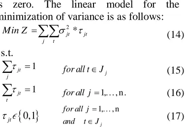
3.2.3. Final modeling and unique ranking
𝜏𝑗𝑡 = 1, unit j has rank t, and in otherwise
is zero. The linear model for the minimization of variance is as follows:
2* jt jt j t
Min Z
(14)
s.t.
1
jt j
for all tJj (15)1
jt t
for all j 1, , n. (16)
0,1jt
1, , n
j
for all j and t J
(17)
The (14) statement, as an objective function, tries to reduce the total variances. Eq. (15) ensures that the rank of each interval is selected as the unique rank. Eq. (16) supports all units in the ranking, in other words, assigns one to each units. Finally, the binary variable is defined. In the next part, with the presentation of a case study, the proposed approach will be used and evaluated.
4. Case Study
Due to the role of banking system in economic growth, unemployment and inflation control, the banking system is one of the most important economic pillars in many countries. Therefore, efficiency analysis is considered as a suitable measure for assessing the firms’ efficiency in this industry. One of the most important issues that make senior executives of banks often fail to implement programs and efficiency evaluation methods in their organization is the program’s disproportion to their needs. On the other hand, with increasing the disclosure of the monetary development crucial role and monetary markets, especially banks in support of the real sector and ultimately, the development and prosperity of the economy, the banks financial system’s reform has become more concern for the country makers attention. Therefore, it was imperative to evaluate this industry by employing basic DEA models with GP and the proposed models. For this reason, 18
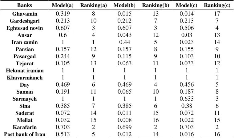
banks that have been most welcomed by the Iranian banks are being evaluated. But one of the problems in determining inputs and outputs is that in most cases there is no information about them, which makes it difficult to decide on inputs and outputs in the studies that are about the efficiency evaluation of banking units by DEA method. Two important factors in the selection of input and output variables are effective: research purpose and, statistical constraints and sample size. Regarding the literature review, with the subject of evaluating the efficiency of bank branches by DEA method and viewing inputs and outputs of these papers, we considered four inputs and two outputs. The input and output variables are introduced in Table 1. Now, the data of each Iranian bank for 2016 is based on four outputs: number of personnel, number of branches, capital (billion rials) and, general and administrative costs (billion rials), and two inputs: net profit (billion rials) and risk. In this case, the risk is an undesirable output because we seek to reduce it, not increase it. To solve this problem, we consider reversal of risk values in place of risk in the output. But in net profit, there are some negative numbers that represent losses. To overcome this problem, another method is used to reduce unpredictable data in the model. After solving the problem of undesired data, the data is presented in Table 2. After solving the problem of undesired data, we put the data in A, B, and C models. The efficiency of each bank in each model is shown in Table 3 and Figure 2.
67
assessment of banks. For example, Iran Zamin Bank based on model (a) has performance 1 and rank 1, it has a performance of 0.44 and a rating of 5 based on model (b) and it has a performance of 0.023 and a rating of 14 based on model (c),. The key question is that "what is the efficiency and rating for this bank?" As stated, the underlying problem is that we do not know how much for banks efficiency should be introduced, since in most cases, the performance based on each model is different with other models. On the other hand, these models are unfairly determined by efficiency and ranking. They do not consider inter-model states. Modalities in which efficient units may be inefficient and inefficient units may be efficient. The novel efficiency ranking approach tries to investigate all existing states between the original GPDEA models that have not been addressed so far. The purpose of these two proposed models is to study the floating mode between the basic models. Also, based on a new structure, we present unique efficiency from each proposed models.
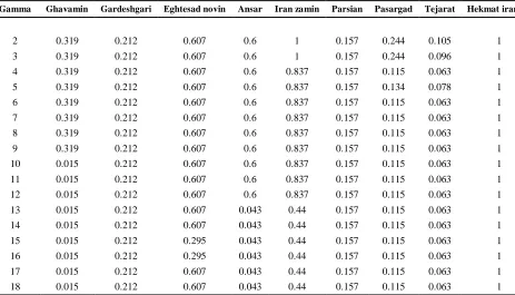
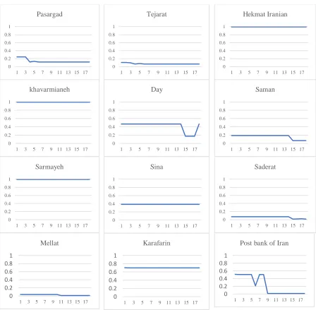
Table 4 and Table 5 show the results of solving the Minisum-SDV model for different gamma values for all units and Table 6 and Table 7 show the results of solving the Minimax-SDV model, too. Minisum-SDV models are run by GAMS for 324 times.The results of the model show 18 efficiencies per banks for different gamma. While our goal was to introduce a number as an efficiency to provide a proper ranking of banks. To solve this problem, taking into account that for each bank 18 efficiency has been obtained, we can draw the performance chart of each bank. In these diagrams, the horizontal axis, gamma variations and vertical axis shows efficiency. The bank efficiency charts for gamma variations are plotted in Figure 3 and Figure 4.
To achieve an efficiency for each bank, the area under each bank's graph is calculated. The maximum area occurs when the efficiency of a unit for all gamma is one. In case of being efficient, for all gamma values, the area will be 1 * (18-1). But we know that the numerical efficiency is [0,1], so we use the following equation: 𝑒𝑓𝑓𝑖𝑐𝑖𝑒𝑛𝑐𝑦𝑖=
𝑏𝑎𝑛𝑘𝑖′𝑠 𝑎𝑟𝑒𝑎
𝑚𝑎𝑥𝑖𝑚𝑢𝑚 𝑎𝑟𝑒𝑎. The area of
each chart and the efficiency of each bank are shown in Table 8.
Given the rankings obtained from the
Minisum-SDV and Minimax-SDV
the performance of a particular unit indicates the imbalance of these models. On the other hand, these models are unfairly determined by performance and ranking. They do not consider inter-model states. Modalities in which efficient units may be inefficient and inefficient units may be efficient. The novel efficiency ranking approach tries to investigate all existing states between the original GPDEA models that have not been addressed so far.
The proposed approach seeks to genuinely determine the ratings of decision-making units in order to obtain an accurate picture of the status quo. In the new approach to performance rating, floating modes are checked between base models to avoid bias in ranking. In this approach, for the change of the gama parameter, which depends on the number of DMUs, all possible modes for determining the efficiency are examined. And for each unit, performance is achieved for all units. After charting each unit, calculating the area of the sub-graph and normalizing it, the unit performance is obtained for each of the Minisum-SDV and Minimax-SDV models. But there is still a multi-level problem for each unit. In order to solve this problem, the rankings obtained from the two suggested models create intervals. These intervals are plotted in Gantt chart, and the variance of each rank is calculated for each unit. After extraction of variances, this time is placed in another linear model. This model tries to select ratings with the least variance from the average of the defined interval. In the end, the ratings of the banks are realistic and taking into account all possible modes.
5. Conclusion
Since the introduction of the Data Envelopment Analysis Method by Charles et al. , this method has become an effective tool for evaluation and modeling. In this method, the relative efficiency of each decision making unit is equal to the
rational ratio of outputs to inputs. The disadvantage of this method is that the number of units evaluated is related to the number of input and output variables. That is, the higher the number of problem variables, the base models have less power to distinguish between efficient and non-working units. Also, when the number of organizational units is less than a certain amount, the power of differentiation of the basic models of data envelopment analysis decreases. In this research, based on the concepts of the ideal planning technique, a model is proposed to improve the assessment of the decision-making units effeciency . The model can solve some of the problems of data envelopment analysis models, including the weakness of the resolution of decision-making units, and in this regard, increases the efficiency of these models. To test this model and compare it with the basic model, information from 18 banks with four input vriables and two output variables were used.
69
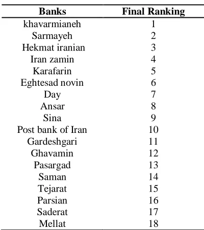
“Mellat” bank also achieved the lowest rank, the eighteenth rank, due to the lowest efficiency level.
For future research, it is suggested that private banks and government banks be compared. Other models of data envelopment analysis, such as network and output models, should be used for current studies and the results should be presented using the proposed model. We hope this research can be used to evaluate different units.
References
[1] H. Y. Aly, R. Grabowski, C. Pasurka and N. Rangan, "Technical, Scale, and Allocative Efficiencies in U.S. Banking: An Empirical Investigation," The Review of Economics and Statistics, vol. 72, pp. 211-218, 1990.
[2] S. M. Miller and A. G. Noulas, "The technical efficiency of large bank production," Journal of Banking & Finance, vol. 20, no. 3, pp. 495-509, 1996.
[3] D. C. Wheelock and P. W. Wilson, "Technical Progress, Inefficiency, and Productivity Change in U.S. Banking, 1984-1993," Journal of Money, Credit and Banking, vol. 31, pp. 212-234, 1999.
[4] H. Bal, H. H. Örkcü and S. Çelebioğlu, "Improving the discrimination power and weights dispersion in the data envelopment analysis," Computers & Operations Research, vol. 37, no. 1, pp. 99-107, 2010.
[5] Y.-H. Chiu and Y.-C. Chen, "The analysis of Taiwanese bank efficiency:
Incorporating both external
environment risk and internal risk," Economic Modelling, vol. 26, no. 2, pp. 456-463, 2009.
[6] D. Holod and H. F. Lewis, "Resolving the deposit dilemma: A new DEA bank efficiency model," Journal of Banking & Finance, vol. 35, no. 11, pp. 2801-2810, 2011.
[7] G. E. Halkos and N. G. Tzeremes, "Estimating the degree of operating efficiency gains from a potential bank merger and acquisition: A DEA
bootstrapped approach," Journal of Banking & Finance, vol. 37, no. 5, pp. 1658-1663, 2013.
[8] H. BAL and H. H. ÖRKÇÜ, "A Goal Programming Approach to Weight Dispersion in Data Envelopment Analysis," G.U.Journal of Science, vol. 20, no. 4, pp. 117-125, 2007.
[9] J. Puri and S. P. Yadav, "A fuzzy DEA model with undesirable fuzzy outputs and its application to the banking sector in India," Expert Systems with Applications, vol. 41, no. 14, pp. 6419-6432, 2014.
[10] I. E. Tsolas and D. I. Giokas, "Bank branch efficiency evaluation by means of least absolute deviations and DEA," Managerial Finance, vol. 38, no. 8, pp. 768-785, 2012.
[11] S. R. Moghadam , S. K. Ghartemani, N. Abbaspoor and A. Shekarchizadeh, "Presentation a Model for Integration of Fuzzy Data Envelopment Analysis and Goal Programming," International Journal of Academic Research in Management (IJARM), vol. 2, pp. 2322-2360, 2013.
[12] J. Johnes, M. Izzeldin and V. Pappas, "A comparison of performance of Islamic and conventional banks 2004–2009," Journal of Economic Behavior & Organization, vol. 103, pp. S93-S107, 2014.
71
[14] L. M. Seiford and J. Zhu, "Profitability and Marketability of the Top 55 U.S. Commercial Banks," Management science, vol. 45, no. 9, pp. 1270-1288, 1999.
[15] A. Charnes, W. Cooper and E. Rhodes, "Measuring the efficiency of decision making units," European Journal of Operational Research, vol. 2, no. 6, pp. 429-444, 1978.
[16] L. Halme, J.-P. Mecklin, M. Juhola, R. Rees and A. Palmu, "Primary Gastrointestinal Non-Hodgkin's Lymphoma: A Population Based Study in Central Finland in 1975–1993," Acta oncologica, vol. 36, no. 1, pp. 69-74, 1997.
[17] X. B. Li and G. R. Reeves, "A multiple criteria approach to data envelopment analysis," European Journal of Operational Research, vol. 115, no. 3, pp. 507-517, 1999.
[18] V. Belton and S. P. Vickers, "Demystifying DEA-A Visual Interactive Approach Based on Multiple Criteria Analysis," The Journal of the Operational Research Society, vol. 44, pp. 883-896, 1993.
[19] T. J. Stewart, "Relationships between Data Envelopment Analysis and Multicriteria Decision Analysis," Journal of the Operational Research Society, vol. 47, no. 5, pp. 654-665, 1996.
[20] J. Zhu, Quantitative models for
performance evaluation and
benchmarking: data envelopment
analysis with spreadsheets,
Massachusetts: Springer, 2014.
[21] Peykani, P., Mohammadi, E., Jabbarzadeh, A., & Jandaghian, A. , "Utilizing robust data envelopment analysis model for measuring efficiency of stock, a case study: Tehran stock exchange," Journal of New Research in Mathematics, vol. 1, no. 4, pp. 15-24, 2016.
[22] Peykani, P., Mohammadi, E. "Interval network data envelopment analysis model for classification of investment companies in the presence of uncertain data," Journal of Industrial and Systems Engineering, no. 11, pp. 63-72, 2018.
[23] Peykani, P., Mohammadi, E., Pishvaee, M. S., Rostamy-Malkhalifeh, M., Jabbarzadeh, A., "A novel fuzzy data envelopment analysis based on robust possibilistic programming: possibility, necessity and credibility-based approaches.," RAIRO-Operations Research, vol. 52, no. 4, pp. 1445-1463, 2018.
[24] Peykani, P., Mohammadi E.,
Rostamy-Malkhalifeh, M., and
Hosseinzadeh Lotfi, F. "Fuzzy Data Envelopment Analysis Approach for Ranking of Stocks with an Application to Tehran Stock Exchange," Advances in Mathematical Finance and Applications, vol. 4, no. 1, pp. 31-43, 2019.
[25] Peykani P, Mohammadi E, Emrouznejad A, Pishvaee MS, Rostamy-Malkhalifeh M, "Fuzzy Data Envelopment Analysis: An Adjustable Approach," Expert Systems with Applications, 2019.
73
Table 1. Input & Output Variables
Inputs
number of Staff 𝑥1 number of branches 𝑥2
Capital 𝑥3
General and administrative costs 𝑥4
outputs net profit 𝑦1
Risk 𝑦2
Table 2. Banks' data
Row Banks Inputs Outputs
Nu. of Staff Nu. of branches capital costs net profit risk
1 Ghavamin 6,783 734 5,182 8,000 683 0.478
2 Gardeshgari 1,055 83 1,433 6,000 143 0.240
3 Eghtesad novin 3,169 282 4,668 11,312 21,269 1.075
4 Ansar 5,217 636 3,775 8,000 2,650 0.885
5 Iran zamin 2,183 327 941 4,000 26,877 0.346
6 Parsian 4,405 294 5,556 23,760 1,820 0.690
7 Pasargad 3,815 327 6,495 50,400 12,047 0.971
8 Tejarat 18,734 1,661 10,171 45,700 24,499 0.280
9 Hekmat iranian 1,137 132 1,053 4,000 828 0.752
10 Khavarmianeh 349 16 615 4,000 2,023 0.917
11 Day 1,007 91 2,819 6,400 2,031 0.549
12 Saman 2,475 143 3,708 8,000 824 0.281
13 Sarmayeh 1,349 143 1,215 4,000 26,303 0.476
14 Sina 2,405 257 2,765 10,000 1,638 0.714
15 Saderat 30,676 2,578 32,742 57,800 1 0.787
16 Mellat 21,177 1,581 37,763 50,000 3,982 0.258
17 Karafarin 1,908 107 1,945 8,500 604 1.124
18 Post bank of Iran 2,952 406 2,946 3,233 2 0.312
Table 3. Banks’ efficiency and ranking under basic models
Banks Model(a) Ranking(a) Model(b) Ranking(b) Model(c) Ranking(c) Ghavamin 0.319 8 0.015 13 0.014 17
Gardeshgari 0.213 10 0.212 7 0.213 7
Eghtesad novin 0.607 3 0.607 3 0.506 4
Ansar 0.6 4 0.043 12 0.03 13
Iran zamin 1 1 0.44 5 0.023 14
Parsian 0.157 12 0.157 8 0.155 9
Pasargad 0.244 9 0.115 9 0.103 10
Tejarat 0.105 13 0.063 11 0.033 12
Hekmat iranian 1 1 1 1 1 1
Khavarmianeh 1 1 1 1 1 1
Day 0.469 6 0.469 4 0.456 5
Saman 0.191 11 0.065 10 0.187 8
Sarmayeh 1 1 1 1 0.633 3
Sina 0.385 7 0.385 6 0.38 6
Saderat 0.072 14 0.011 15 0.072 11
Mellat 0.032 15 0.008 16 0.022 15
Karafarin 0.703 2 0.699 2 0.703 2
Figure 2. Banks’ Efficiency under basic models
Table 4. Banks’ efficiency under Minisum-SDV
Gamma Ghavamin Gardeshgari Eghtesad novin Ansar Iran zamin Parsian Pasargad Tejarat Hekmat iranian
2 0.319 0.212 0.607 0.6 1 0.157 0.244 0.105 1
3 0.319 0.212 0.607 0.6 1 0.157 0.244 0.096 1
4 0.319 0.212 0.607 0.6 0.837 0.157 0.115 0.063 1
5 0.319 0.212 0.607 0.6 0.837 0.157 0.134 0.078 1
6 0.319 0.212 0.607 0.6 0.837 0.157 0.115 0.063 1
7 0.319 0.212 0.607 0.6 0.837 0.157 0.115 0.063 1
8 0.319 0.212 0.607 0.6 0.837 0.157 0.115 0.063 1
9 0.319 0.212 0.607 0.6 0.837 0.157 0.115 0.063 1
10 0.015 0.212 0.607 0.6 0.837 0.157 0.115 0.063 1
11 0.015 0.212 0.607 0.6 0.837 0.157 0.115 0.063 1
12 0.015 0.212 0.607 0.6 0.837 0.157 0.115 0.063 1
13 0.015 0.212 0.607 0.043 0.44 0.157 0.115 0.063 1
14 0.015 0.212 0.607 0.043 0.44 0.157 0.115 0.063 1
15 0.015 0.212 0.295 0.043 0.44 0.157 0.115 0.063 1
16 0.015 0.212 0.295 0.043 0.44 0.157 0.115 0.063 1
17 0.015 0.212 0.607 0.043 0.44 0.157 0.115 0.063 1
18 0.015 0.212 0.607 0.043 0.44 0.157 0.115 0.063 1
0 0.2 0.4 0.6 0.8 1 1.2
75
Table 5. Banks’ efficiency under Minisum-SDV
Gamma khavarmianeh Day Saman Sarmayeh Sina Saderat Mellat Karafarin Post bank of Iran
2 1 0.469 0.191 1 0.385 0.072 0.032 0.699 0.507
3 1 0.469 0.191 1 0.385 0.072 0.032 0.699 0.507
4 1 0.469 0.191 1 0.385 0.072 0.032 0.699 0.507
5 1 0.469 0.191 1 0.385 0.072 0.032 0.699 0.507
6 1 0.469 0.191 1 0.385 0.072 0.032 0.699 0.211
7 1 0.469 0.191 1 0.385 0.072 0.032 0.699 0.507
8 1 0.469 0.191 1 0.385 0.072 0.032 0.699 0.507
9 1 0.469 0.191 1 0.385 0.072 0.032 0.699 0.012
10 1 0.469 0.191 1 0.385 0.072 0.032 0.699 0.012
11 1 0.469 0.191 1 0.385 0.072 0.008 0.699 0.012
12 1 0.469 0.191 1 0.385 0.072 0.008 0.699 0.012
13 1 0.469 0.191 1 0.385 0.072 0.008 0.699 0.012
14 1 0.469 0.191 1 0.385 0.072 0.008 0.699 0.012
15 1 0.172 0.065 1 0.385 0.011 0.008 0.699 0.012
16 1 0.172 0.065 1 0.385 0.017 0.008 0.699 0.012
17 1 0.172 0.065 1 0.385 0.019 0.008 0.699 0.012
18 1 0.469 0.065 1 0.385 0.011 0.008 0.699 0.012
Table 6. Banks’ efficiency under Minimax-SDV
Gamma Ghavamin Gardeshgari Eghtesad
novin Ansar Iran
zamin Parsian Pasargad Tejarat
Hekmat iranian
2 0.319 0.213 0.607 0.6 0.587 0.157 0.244 0.105 1
3 0.319 0.213 0.607 0.5 1 0.157 0.244 0.105 1
4 0.319 0.212 0.607 0.6 0.909 0.157 0.195 0.105 0.911
5 0.319 0.212 0.607 0.6 0.605 0.157 0.181 0.105 1
6 0.319 0.163 0.31 0.199 0.579 0.157 0.181 0.105 0.958
7 0.319 0.131 0.335 0.117 0.562 0.105 0.181 0.105 1
8 0.319 0.004 0.16 0.03 0.472 0.012 0.118 0.105 0.989
9 0.319 0.004 0.16 0.03 0.472 0.012 0.118 0.105 0.333
10 0.319 0.004 0.16 0.03 0.44 0.012 0.205 0.105 0.923
11 0.005 0.004 0.16 0.03 0.44 0.012 0.181 0.105 0.121
12 0.005 0.004 0.16 0.386 0.44 0.012 0.181 0.105 0.121
13 0.005 0.212 0.6 0.533 0.457 0.012 0.181 0.105 0.234
14 0.091 0.163 0.31 0.124 0.478 0.012 0.118 0.105 0.546
15 0.069 0.131 0.335 0.117 0.491 0.012 0.181 0.105 0.357
16 0.005 0.004 0.16 0.03 0.447 0.012 0.118 0.105 0.028
17 0.015 0.212 0.607 0.043 0.44 0.157 0.115 0.079 0.121
Table 7. Banks’ efficiency under Minimax-SDV
Gamma khavarmianeh Day Saman Sarmayeh Sina Saderat Mellat Karafarin Post bank of Iran
2 1 0.366 0.191 0.454 0.385 0.072 0.032 0.477 0.239
3 1 0.469 0.191 1 0.385 0.072 0.032 0.699 0.042
4 1 0.469 0.191 1 0.385 0.072 0.032 0.699 0.056
5 1 0.469 0.191 0.774 0.385 0.072 0.032 0.699 0.507
6 1 0.469 0.191 0.654 0.385 0.072 0.032 0.699 0.507
7 1 0.172 0.065 1 0.244 0.072 0.032 0.45 0.11
8 1 0.469 0.066 1 0.207 0.072 0.032 0.432 0.239
9 1 0.025 0.008 1 0.021 0.072 0.032 0.011 0.213
10 1 0.025 0.008 1 0.021 0.072 0.032 0.011 0.163
11 1 0.025 0.008 1 0.021 0.072 0.032 0.699 0.122
12 1 0.438 0.008 1 0.021 0.072 0.032 0.699 0.252
13 1 0.469 0.191 1 0.021 0.072 0.032 0.699 0.056
14 1 0.172 0.065 1 0.244 0.072 0.032 0.327 0.054
15 1 0.177 0.066 1 0.207 0.072 0.032 0.432 0.056
16 1 0.025 0.008 0.758 0.021 0.072 0.032 0.011 0
17 1 0.469 0.191 1 0.385 0.072 0.032 0.699 0.012
18 1 0.456 0.187 0.633 0.38 0.072 0.022 0.703 0.016
Figure 3. Bank efficiency charts under Minisum-SDV model
0 0.2 0.4 0.6 0.8 1
1 3 5 7 9 11 13 15 17
Ghavvamin
0 0.2 0.4 0.6 0.8 1
1 3 5 7 9 11 13 15 17
Gardeshgari
0 0.2 0.4 0.6 0.8 1
1 3 5 7 9 11 13 15 17
Eghtesad novin
0 0.2 0.4 0.6 0.8 1
1 3 5 7 9 11 13 15 17
Ansar
0 0.2 0.4 0.6 0.8 1
1 3 5 7 9 11 13 15 17
Iran zamin
0 0.2 0.4 0.6 0.8 1
1 3 5 7 9 11 13 15 17
77
Figure 4. Bank efficiency charts under Minimax-SDV model
0 0.2 0.4 0.6 0.8 1
1 3 5 7 9 11 13 15 17
Pasargad 0 0.2 0.4 0.6 0.8 1
1 3 5 7 9 11 13 15 17
Tejarat 0 0.2 0.4 0.6 0.8 1
1 3 5 7 9 11 13 15 17
Hekmat Iranian 0 0.2 0.4 0.6 0.8 1
1 3 5 7 9 11 13 15 17
khavarmianeh 0 0.2 0.4 0.6 0.8 1
1 3 5 7 9 11 13 15 17
Day 0 0.2 0.4 0.6 0.8 1
1 3 5 7 9 11 13 15 17
Saman 0 0.2 0.4 0.6 0.8 1
1 3 5 7 9 11 13 15 17
Sarmayeh 0 0.2 0.4 0.6 0.8 1
1 3 5 7 9 11 13 15 17
Sina 0 0.2 0.4 0.6 0.8 1
1 3 5 7 9 11 13 15 17
Saderat 0 0.2 0.4 0.6 0.8 1
1 3 5 7 9 11 13 15 17
Mellat 0 0.2 0.4 0.6 0.8 1
1 3 5 7 9 11 13 15 17
Karafarin 0 0.2 0.4 0.6 0.8 1
1 3 5 7 9 11 13 15 17
Post bank of Iran
0 0.2 0.4 0.6 0.8 1
1 3 5 7 9 11 13 15 17
Ghavamin 0 0.2 0.4 0.6 0.8 1
1 3 5 7 9 11 13 15 17
Gardeshgari 0 0.2 0.4 0.6 0.8 1
1 3 5 7 9 11 13 15 17
0 0.2 0.4 0.6 0.8 1
1 3 5 7 9 11 13 15 17
Ansar 0 0.2 0.4 0.6 0.8 1
1 3 5 7 9 11 13 15 17
Iran zamin 0 0.2 0.4 0.6 0.8 1
1 3 5 7 9 11 13 15 17
Parsian 0 0.2 0.4 0.6 0.8 1
1 3 5 7 9 11 13 15 17
Pasargad 0 0.2 0.4 0.6 0.8 1
1 3 5 7 9 11 13 15 17
Tejarat 0 0.2 0.4 0.6 0.8 1
1 3 5 7 9 11 13 15 17
Hekmat 0 0.2 0.4 0.6 0.8 1
1 3 5 7 9 11 13 15 17
Khavaremiane 0 0.2 0.4 0.6 0.8 1
1 3 5 7 9 11 13 15 17
Day 0 0.2 0.4 0.6 0.8 1
1 3 5 7 9 11 13 15 17
Saman 0 0.2 0.4 0.6 0.8 1
1 3 5 7 9 11 13 15 17
Sarmaye 0 0.2 0.4 0.6 0.8 1
1 3 5 7 9 11 13 15 17
Sina 0 0.2 0.4 0.6 0.8 1
1 3 5 7 9 11 13 15 17
Saderat 0 0.2 0.4 0.6 0.8 1
1 3 5 7 9 11 13 15 17
Mellat 0 0.2 0.4 0.6 0.8 1
1 3 5 7 9 11 13 15 17
Karafarin 0 0.2 0.4 0.6 0.8 1
1 3 5 7 9 11 13 15 17
79
Table 8. The area of each chart and the efficiency of each bank under Minisum-SDV and Minimax-SDV
Banks Minisum-SDV Minimax-SDV area efficiency rank area efficiency rank
Ghavamin 2.839 0.167 10 2.38 0.14 12
Gardeshgari 3.604 0.212 8 2.091 0.123 13
Eghtesad Novin 8.993 0.529 4 6.443 0.379 6
Ansar 7.089 0.417 5 4.284 0.252 8
Iran Zamin 12.444 0.732 2 9.333 0.549 4
Parsian 2.669 0.157 12 1.309 0.077 16
Pasargad 2.244 0.132 13 2.567 0.151 11
Tejarat 1.547 0.091 14 1.717 0.101 15
Hekmat iranian 17 1 1 10.727 0.631 3
khavarmianeh 17 1 1 17 1 1
Day 6.732 0.396 6 5.168 0.304 7
Saman 2.805 0.165 11 1.819 0.107 14
Sarmayeh 17 1 1 15.691 0.923 2
Sina 6.545 0.385 7 3.536 0.208 9
Saderat 1.037 0.061 15 1.224 0.072 17
Mellat 0.357 0.021 16 0.527 0.031 18
Karafarin 11.883 0.699 3 8.415 0.495 5
Post bank of Iran 3.604 0.212 9 2.839 0.167 10
Figure 5. Gantt chart
1 2 3 4 5 6 7 8 9 10 11 12 13 14 15 16 17 18
Ghavamin [10,12] 1.67 0.67 1.67
Gardeshgari [8,13] 9.17 5.17 3.17 3.17 5.17 9.17
Eghtesad novin [4,6] 1.67 0.67 1.67
Ansar [5,8] 3.5 1.5 1.5 3.5
Iran zamin [2,4] 1.67 0.67 1.67
Parsian [12,16] 6 3 2 3 6
Pasargad [13,11] 1.67 0.67 1.67
Tejarat [14,15] 0.5 0.5
Hekmat iranian [1,3] 1.67 0.67 1.67
khavarmianeh [1,1] 0
Day [6,7] 0.5 0.5
Saman [11,14] 3.5 1.5 1.5 3.5
Sarmayeh [1,2] 0.5 0.5
Sina [7,9] 1.67 0.67 1.67
Saderat [15,17] 1.67 0.67 1.67
Mellat [16,18] 1.67 0.67 1.67
Karafarin [3,5] 1.67 0.67 1.67
Post bank of Iran [9,10] 0.5 0.5
Banks Interval
ranking
Table 9. Final banks’ ranking
Banks Final Ranking
khavarmianeh 1
Sarmayeh 2
Hekmat iranian 3
Iran zamin 4
Karafarin 5
Eghtesad novin 6
Day 7
Ansar 8
Sina 9
Post bank of Iran 10
Gardeshgari 11
Ghavamin 12
Pasargad 13
Saman 14
Tejarat 15
Parsian 16
Saderat 17