Analyzing Stop Time Phase Leading to Congestion Based on Drivers’ Behavior Patterns

(1)

383 International Journal of Transportation Engineering, Vol.5/ No.4/ Spring 2018

Analyzing Stop Time Phase Leading to Congestion Based on

Drivers’ Behavior Patterns

Babak Mirbaha

1

, Ali Abdi Kordani

2

, Arsalan Salehikalam

3

, Mohammad Zarei

4

Received: 11.07.2016 Accepted: 16.07.2017

Abstract

Traffic oscillation, stop and go traffic, is created by different reasons such as: sudden speed drop of leader vehicle. Stop and go traffic commonly is observed in congested freeways results in traffic oscillation. Many theories had been presented to define congestion traffic based on laws of physics such as: thermodynamics and fluid. But, these theories could not explain the complexity of driving responses in different situations of traffic especially in traffic jams. Unfortunately, because trajectories data are very scarce, our understanding of this type of oscillations in congested traffic is still limited. When the leader vehicle of a platoon drops speed, deceleration waves are released from downstream to upstream. Follower vehicles reacts different behavioral reactions based on personal characteristics. In this paper, behavioral patterns of follower driver were classified based on asymmetric microscopic driving behavior theory and traffic hysteresis in NGSIM trajectories. They were four patterns in deceleration phase and two patterns in acceleration phase. Then, two parameters of last deceleration wave leading to congestion, time and space parameters, τ and δ, were calculated based on Newell’s car following model. Time of two phases, stop and congestion phases, were identified based on follower vehicle trajectory. In order to calculate time of two phases, two points were identified: point of receiving stop wave leading to congestion and point of entering to congestion. Artificial neural network models were developed to analyze the relationship between the microscopic parameters and time of two phases. Analysis results present spacing difference of follower between stop and congestion phase based on under reaction-timid pattern and spacing difference of follower between deceleration and congestion phase based on over reaction-timid pattern and spacing of leader vehicle at the wave diffusion point are most effective parameters in stop time leading to congestion. One of the main practical applications of this paper can be the addressing one of the main problems of micro simulation soft wares (like Aimsun) due to behavioral patterns.

Keywords: Stop time lead to congestion; Stop and go traffic; NGSIM data trajectory; Behavior patterns; Artificial neural networks

Corresponding author E-mail: [email protected]

1

Assistant Professor, Faculty of Engineering, Imam Khomeini International University, Qazvin, Iran. 2 Assistant Professor, Faculty of Engineering, Imam Khomeini International University, Qazvin, Iran. 3 PHD candidate, Imam Khomeini International University, Qazvin, Iran.

(2)

Analyzing Stop Time Phase Leading to Congestion based on Drivers’ Behavior patterns

1. Introduction

Sudden speed drop of vehicles in freeways results in stop and go traffic. It has negative effects such as: delay, increasing fuel consumption and safety hazards. Traffic oscillation is developed by reasons such as lane change maneuvers and moving bottlenecks [ Zheng et al. 2011a; Chen et al., 2012; Bilbao- Ubillos, 2008; Zheng et al. 2011b; Ahn and Cassidy, 2007; Laval and Daganzo, 2006; Koshi, Kuwahara and Akahane, 1992; Laval, 2006 ]. Traffic oscillation results in propagation and grow kinematic waves from downstream to upstream in the vehicles' platoon [Mauch and Cassidy, 2002]. Due to these various factors, it is important to model stop and go traffic and understand the shape and type of propagation of this type of oscillation in congested traffic. Unfortunately, due to lack or scarce detailed vehicle trajectories and aggregated sensor data, our understanding about micro behavior characteristics of moving vehicles in traffic is still limited. Newell proposed the first theory for explaining driver asymmetric behavior. It is based on two separate curves for acceleration and deceleration of spacing – velocity. He showed that the spacing in acceleration is always larger than the deceleration for the same speed [Yeo and Skabardonis, 2009]. Also, Newell considered parallel trajectories of leader and follower vehicles. The wave speeds were also assumed similar for two phases of acceleration and deceleration. But, his approach wasn’t complete to describe life cycle, generation and growth wave in vehicle platoon [Newell, 2002]. Del Castillo considered the same wave speeds. He analyzed life cycle of stop and go traffic in congestion. His researches presented that waves grow in dense traffic flow and cause delay in low density flow. In other hand, if there is congested traffic, traffic oscillation grows [Castillo, 2001]. Kim and Zhang calculated waves with different speeds for acceleration and deceleration phases. They used stochastic gap time and assumed gap time completely stochastic for any driver. They assumed that data trajectories are parallel [Kim and Zhang, 2004]. Yeo and Skabardonis presented a microscopic asymmetric theory based

(3)

Babak Mirbaha, Ali Abdi Kordani, Arsalan Salehikalam, Mohammad Zarei

385 International Journal of Transportation Engineering, Vol.5/ No.4/ Spring 2018 flows based on driver behavior. The

speed-density curve was divided into three traffic phases; namely, relaxation phase in acceleration pattern, prediction phase in deceleration pattern, prediction- relaxation balanced phase in strong equilibrium. He demonstrated an increase in driver concentration on acceleration pattern, and reduction in driver concentration in the deceleration phase [Zhang, 1999]. Zhang and Kim applied a new car-following theory in which new variables were introduced and used; such as, gap time as a function of gap distance, and traffic phase including acceleration, deceleration and coasting condition [Zhang and Kim, 2006]. Laval presented that hysteresis magnitude estimation is based on measurements taken during non-steady state conditions in previous studies that resulted in measurement error. He used NGSIM trajectories and hysteresis phenomena magnitude in invariable density and classified into four levels: Strong, Weak, Negligible and Negative level. Also, his research shows that different driver behaviors cause separate loops of flow – density plot in deceleration and acceleration phases. These loops present timid maneuver, clockwise loop of speed – spacing plot, and aggressive maneuver, counter-clockwise loop of speed – spacing plot [Laval, 2010]. Ahan et al analyzed the evolution of speed-spacing relationships as vehicles exit from stop-and-go oscillations based on the kinematic wave model with variable wave speed. They used equilibrium spacing instead of observed spacing. Their researches show that hysteresis magnitude takes place less frequently and in smaller amplitude than previously thought [Ahn, Vadlamani and Laval, 2013]. Chen et al presented a behavioral car-following model based on NGSIM trajectories. Their model was able to reproduce the spontaneous formation and ensuing propagation of stop and go waves in traffic oscillation. The statistical results of their model reveal that traffic oscillation depends on driver behavior. Also, we have to consider this correlation between driver behavior of before and during oscillation [Chen et al., 2012]. Chen et al analyzed traffic hysteresis based on a behavioral car-following model. Their researches presented

that type of traffic hysteresis is dependent on driver behavior when experiencing traffic oscillations but driver behavior is independent on its position along the oscillation. Also, their investigations revealed development in different stages of oscillation, growth and fully-developed, depending on the different patterns of hysteresis and driver behavior characteristics [Chen et al., 2012]. Orfanou et al. extend past investigations about oscillation by identifying traffic hysteresis. Using Trajectory Explorer software and artificial neural networks, hysteresis characteristics were analyzed based on classifying phenomena behavioral perspectives, aggressive and timid, at the microscopic level. Analysis of results of artificial neural networks presented that changes in the two parameters, spacing and acceleration at the end of the phenomenon, are the most critical determinants [Orfanou, Vlahogianni and Karlaftis, 2012]. Mohsen Poor Arab Moghadam et al, presented a car-following model that developed combining an Adaptive Neuro-Fuzzy Inference System (ANFIS) and a Classification And Regression Tree (CART). It simulated the reaction time of follower behavior of each driver-vehicle-unit (DVU). Their results were compared with Ozaki’s reaction time[Mohsen Poor Arab Moghadam et al., 2016]. In this paper, different behavior patterns of following driver are classified based on maneuvering errors in deceleration phase and based on traffic hysteresis, aggressive and timid, in acceleration phase. Then we calculated time between two phases based on the deceleration wave leading to congestion in traffic oscillation. Also, artificial neural network models are developed to approximate the microscopic characteristics of behavior diversion at the microscopic level and different categories of driver patterns in deceleration and deceleration phases.

2. Research Methodology

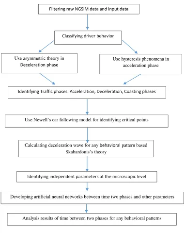
In order to better express the methodological pattern of this study, Figure 1 shows the order and different parts of the methodology used in this paper.

(4)

In this research, NGSIM data are divided into four behavioral patterns based on the performance errors of the follower driver, which are under reaction with under constant reaction and over constant reaction in the deceleration phase leading to congestion and based on the hysteresis phenomenon in the acceleration phase into two behavioral patterns of aggressive and timid drivers. As the follower vehicle leaves the traffic oscillation, the behavior of the aggressive (timid) driver indicates that the faster (slower) reaction of the follower vehicle driver than the driver's behavior of the Newell's car following model leads to a higher (lower) leading vehicle distance diagram than the Newell vehicle's diagram at the macroscopic level (space-time curve). In other words, the propagation of the wave velocity in the acceleration phase between the vehicles in the platoon is done at a faster (slower) speed and a less (more) reaction time. At the microscopic level, the behavior of the aggressive (timid) driver leads to the formation of counter-clockwise (clockwise) circles in the space-velocity curve. According to the statistical results of the behavioral patterns of the following vehicle driver in Table 1 and based on the analysis of 544 coupling platoons leading up to the congestion, this study had examined only three behavioral patterns with under-timid reaction, over-timid reaction, and over-timid constant reaction due to the lack of transmitted data.

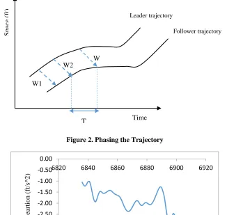
2.2 Phasing the Trajectory

As shown in Figure2, the follower vehicle trajectory was classified into three phases: the propagation of the deceleration wave leading up to the congestion, entering stop and congestion phase based on the asymmetric behavioral theory and HCM 2010. For determining the start of deceleration phase leading up to the congestion, the acceleration of the follower and leader vehicle in the data trajectory must be less than -1 in order to exit from the coasting phase before deceleration and the speed of follower and leader vehicle starts to slow down to reach zero quickly. As shown in Figure3, in phasing the trajectory, it is possible to accelerate the follower and leader

vehicles in the deceleration phase. In other words, the acceleration of both devices is always less than -1 and spacing is not so much that the follower and leader vehicle can exit the deceleration phase. For this reason, under the influence of the latest wave, the follower vehicle deceleration leading up to the congestion will reach zero under the influence of deceleration. The starting point of the entry to stop phase is considered less than 5 mph based on the HCM 2010, which the follower and leader vehicles decelerates continuously in order to enter the congestion phase, i.e. zero speed. W1: the latest wave of deceleration leading up to the congestion, W2: stop wave, W3: congestion wave, T: the time between two phases of stop and congestion

2.3 Introducing the Parameters

(5)

387 International Journal of Transportation Engineering, Vol.5/ No.4/ Spring 2018 Figure (1): Flowchart of research methodology

Table 1. The Statistical Results of the Behavioral Patterns Behavioral pattern

The number of pairs deceleration phase

patterns Aggressive Timid

Over reaction 295 63 232

Under reaction 129 19 110

Over cotenant reaction 90 6 84

Under cotenant reaction

30 14 16

Platoon total 544 544

Filtering raw NGSIM data and input data

Use asymmetric theory in

Deceleration phase

Identifying Traffic phases: Acceleration, Deceleration, Coasting phases

Use Newell’s car following model for identifying critical points

Calculating deceleration wave for any behavioral pattern based Skabardonis’s theory

Identifying independent parameters at the microscopic level

Developing artificial neural networks between time two phases and other parameters Use hysteresis phenomena in

acceleration phase

Classifying driver behavior

(6)

Figure 2. Phasing the Trajectory

Figure 3. The follower vehicle acceleration-time chart (from the propagation of the deceleration wave until entering the congestion) based on the NGSIM transmitted data

-3.50 -3.00 -2.50 -2.00 -1.50 -1.00 -0.50 0.00

6820 6840 6860 6880 6900 6920

Accele

arti

on

(f

t/

s^

2

)

Time (*0.1 s) W

W1

W2

Sp

ace

(f

t)

Time

T

Leader trajectory

Follower trajectory

Decelera tion Phase

Congestion phase

Space

(f

t)

Time (S) Leader Trajectory

Follower Trajectory

(7)

389 International Journal of Transportation Engineering, Vol.5/ No.4/ Spring 2018 Figure 4. Introducing the Parameters at the Microscopic Level in the Interval-Time Chart

2.4 Artificial Neural Network Model

In a general classification, the vehicles following models are classified into two categories: based on the mathematical relations and input-output models (neural network). In mathematical models, the behavior of the follower vehicle is presented by mathematical relations. In neural network models, the behavior of the follower vehicle is analyzed based on the actual measured values. In these models, inputs and outputs are designed and instructed based on the actual data of the model. The nonlinear behavior of the follower driver leads to the use of intelligent algorithms such as neural network models. Many researchers have used the neural network model in traffic due to the nonlinearity of the driver behavior. Zheng et al., Khodayari et al., Xiaoliang, Hongefi and Panwai have used the neural network model to identify the delay instant reaction in the following vehicle models [Zheng et al., 2013; Khodayari and Ghafari, 2012; Xiaoliang, 2006; Hongefi et al., 2003; Panwai and Dia, 2007 ].

2.4.1 Designing the Neural Network Model

Due to the plurality of parameters and error in the collected data as well as the presence of noise in the sensor of the installed cameras, the neural network model is used in order to identify and analyze the effective parameters of the motion-stop traffic at the microscopic level. The effect of different parameters at the microscopic level on the time between two phases of stop and congestion in different behavioral patterns is identified by using the neural network model. Neural networks are computational models with a large parametric space and specified flexible

structure, which are inspired by neurological studies [Karlaftis and Vlahogianni, 2011] and they are also a practical way to learn various functions as functions with real, discrete and vector values. They are constructed based on interconnecting several processing units, in which neuron is composed of an arbitrary number of nodes or neurons that associate the input with the output. According to table 1, which shows the multilayer perceptron structure in the neural network, this research has used multilayer perceptron networks belonging to the feed-forwards networks based on the error back-propagation learning rule [Orfanou et al., 2012]. The neural network pattern consists of four layers, an input layer, two hidden layers and an output layer. Each layer contains some neurons that receive information from the previous layers and then progress to the next layers and the number of hidden layers neurons are determined by guess and error in order to reach the ideal condition. The multilayer perceptron action as an approximate function results in their advantage than the more complex structures of the neural networks, which it can be directly linked to the statistical model through the correct selection of the operator function [Orfanou et al., 2012]. The structure of the neural network is presented according to Table 2, which the stimulus function of the neural network model is considered as the Tansing function in this research and the methodology for training the neural network model is based on fixing the weights for all variables except for constant input variables after training the neural network mode, moreover, the transmitted data are divided into three sections, as follows: training (70%), Cross – validation (15 %), testing (15%)

Table 2. Structural Characteristics of the Neural Network Model Value

Parameter

Spacing of leader vehicle at the wave propagation point, Sl1

Spacing of leader vehicle at the wave receive point, Sl2

(8)

Spacing of follower vehicle at the wave receive point, Sf2

Input space The difference in spacing of follower vehicle between wave propagation and receive points, ∆S = Sf2−

Sf1

The difference in spacing of leader vehicle between wave propagation and receive points, ∆S𝑙 = Sl2−

Sl1

Spacing difference between two stop and congestion phases, Δ𝑆𝑓2( Jam , Stop)

spacing difference between two congestion and deceleration phases, ΔS(F Jam , Dcc)

The follower vehicle velocity when receiving the stop wave, Vf2

Tansig Architecture

Time of between two phases

Back – propagation Learning rule

2.5 Analyzing the Time Sensitivity between

two Phases of Stop and Congestion

This study has used Crystal Ball software to determine the effect of independent variables on the dependent variables, which it can be connected to the neural network model in the Matlab software by using the Excel software. In this software, the sensitivity of the dependent variable to the independent variable is determined by specifying the uniform probabilities for all independent variables.

2.6 NGSIM Data

This study has used the NGSIM project data, which includes the vehicle ID, line and vehicle position within 0.1 seconds, the temporal and spacing, speed and acceleration of the follower and leader vehicle and their ID [NGSIM, 2006]. Freeway I-80 (US 101) is a 6-lane freeway with a length of 1.650 ft (2100 ft) including a high

occupancy vehicle (HOV) lane. The transmitted data collection and processing in freeway I-80 includes time intervals of (4:00-4:15 pm) and (5:00-5:30 pm) and in freeway US101 contains a time interval of (7:50-8:35 a.m.) with an accuracy of 0.1 seconds. Using the Savitzky and Golay method, the fluctuation of data that were collected from the recorded films in the NGSIM project were filtered and deleted by cameras located on the freeways [Ahn et al., 2011].

3. Analysis of the Results

3.1 Evaluation of The Neural Network

Performance

According to Table 3, evaluating the perceptron performance of the neural network shows that correlation coefficient between the observed and predicted data is presented based on each different behavioral pattern that is also associated with each variable.

Table 3. The Statistical Evaluation of Neural Network Performance

Over reaction constant Over reaction

Under reaction

0.053 0.061

0.056 MSE

0.133 0.133

(9)

391 International Journal of Transportation Engineering, Vol.5/ No.4/ Spring 2018

90 % 92 %

95 %

Percent Correct

Figure 5. Sensitivity Analysis Chart of the Parameters Based on the Behavioral Patterns with Over Reaction- Timid

3.2 The Time Between Two Stop And

Congestion Phases

3.2.1. Over reaction-timid driver

According to Figure5, the results of analyzing the sensitivity of the transmitted data from nine parameters at the microscopic level indicates that three parameters of spacing difference of the follower vehicle between two deceleration and congestion phases, spacing difference of the follower vehicle when propagating and receiving the stop wave, and spacing of the follower vehicle when propagating the stop wave have, respectively the greatest effect on the amount of time between two phases.

3.2.1.1 The Neural Network Models Of

the Parameters Effective On the

Microscopic Level

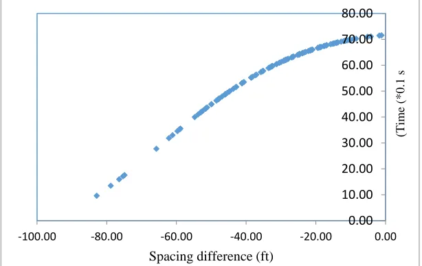
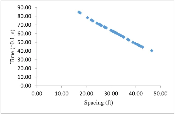
According to Figure6, increasing the spacing difference between acceleration and congestion phases leads to an increase in the time of entering to the stop leading up to the congestion. The

follower driver based on the behavioral pattern with overreaction tends to drive in a safer spacing than the balanced driver, Newell. When a high safety spacing at the time of propagating deceleration wave leading to congestion enters the traffic oscillation, due to the fixing the safe spacing, a higher deceleration, a decrease in time occurs between two phases in order to increase the maneuverability of the traffic oscillation. However, the time increases between two phases by increasing the amount of safe spacing at the time of congestion wave propagation. Increasing the safe spacing of the follower driver in the phase of receiving the deceleration wave leads to increasing the maneuverability of the driver when entering the congestion phase and the driver's less tendency to slow down leads to an increase the time between two phases. In other words, the follower driver provides the safe spacing when entering the stop phase by slowing down the velocity in the phase of receiving deceleration wave, which leads to a lower deceleration in the phase between the stop leading to congestion. As

-30.00 -20.00 -10.00 0.00 10.00 20.00 30.00 40.00 50.00

(10)

the wave is propagated from the leader vehicle, the amount of spacing in the follower vehicle is 𝑆𝑓1 and its amount is equal to 𝑆𝑓2 when it receives the deceleration wave at the point of receiving the wave. If the amount of follower spacing when receiving the deceleration wave is lower than when propagating the deceleration wave, the value of the independent variable, Δ𝑆_𝑓=( 𝑆_𝑓2 - 𝑆_𝑓1) , will be negative.

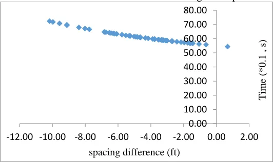
According to Figure7, reducing the spacing difference of the follower vehicle when propagating and receiving the stop wave leads to an increase in the time between stop and congestion phases. Increasing spacing of the

follower vehicle at the time of propagating the stop wave leads to increase the maneuverability and provide the sufficient safe headway. Providing a safe spacing leads to the driver's reluctance to slow down, increasing the time between two phases. Reducing spacing at the time of wave propagation leads to decrease the safe spacing before entering the stop phase as well as increasing spacing when receiving the wave leads to increase the maneuverability of the follower driver in order to supply the lack of safe spacing when entering the stop phase. Thus, the follower driver has more speed drop, reducing the time between two phases, in order to provide the intended safe spacing.

Figure 6. The Neural Pattern of Time based on spacing Difference of the Follower Vehicle between two Deceleration and Congestion Phases

0.00 10.00 20.00 30.00 40.00 50.00 60.00 70.00 80.00

-100.00 -80.00 -60.00 -40.00 -20.00 0.00

Ti

m

e (*

0.

1

s

(

Spacing difference (ft)

0.00 10.00 20.00 30.00 40.00 50.00 60.00 70.00 80.00 90.00

-40.00 -30.00 -20.00 -10.00 0.00 10.00

Tim

e

(*

.1

S

(

(11)

International Journal of Transportation Engineering, 393 Vol.5/ No.4/ Spring 2018

Figure 8. Spacing of the Leader Vehicle when Propagating the Stop Wave

Figure 9. The Chart of analyzing the parameters sensitivity based on the behavioral pattern with under reaction-timid

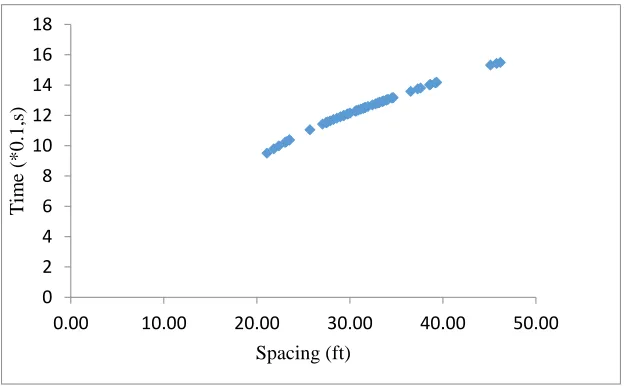
According to Figure 8, increasing the spacing of the leader vehicle when propagating the stop wave leads to an increase in the time between two phases of stop and congestion. Increasing spacing leads to a smoother flow of traffic and providing a safe spacing in the traffic oscillation. Providing a safe spacing leads to driver's reluctance to slow down, increasing the time between the two phases.

3.2.2 Under Reaction- Timid Driver

According to Figure9, the results of analyzing the transmitted data sensitivity from nine parameters at the microscopic level indicates that two parameters of spacing difference of the follower

vehicle between two phases of deceleration and congestion, and spacing of the leader vehicle when propagating the stop wave have the greatest effect on the amount of time between two phases, respectively.

3.2.2.1 The

Artificial Neural Network

Models Of the Parameters Effective On

the Microscopic Level

According to Figure10, increasing the spacing difference between two stop and congestion phases leads to increase the time of entering the stop leading to the congestion. The follower driver based on the behavioral pattern with under reaction tends to drive in spacing with less safety than the balanced driver, Newell. Increasing

0.00 10.00 20.00 30.00 40.00 50.00 60.00 70.00

0.00 10.00 20.00 30.00 40.00 50.00 60.00

Ti

m

e (*

0.

1

,

s)

Spacing (ft)

-20.00 0.00 20.00 40.00 60.00 80.00 SL1

(12)

spacing of the follower vehicle when receiving the stop wave leads to reducing spacing difference. The driver with under reaction does not show reluctance to slow down than the received wave due to the ability to drive at low safety spacing and driver continues to move until the safe spacing decreases to the extent that driver had to lower the velocity more quickly, reduce the time between two phases, in order to provide a safe spacing. Also, increasing spacing of the follower vehicle when receiving the congestion wave leads to increasing spacing difference and the time between two phases. Increasing spacing at congestion indicates that

the follower driver has fewer tendencies to slow down and increase the time between two phases due to the ability to drive in a limited spacing and s/he continues to move in the traffic oscillation with a safe spacing

According to Figure 11, increasing the spacing of the leader vehicle leads to increasing the time between two phases of stop and congestion. Increasing spacing leads to a smooth flow of traffic. The maneuverability of the follower driver increases based on the pattern with under reaction, which leads to the driver's unwillingness to slow down; thus the time for reaching the congestion will increase.

Figure 10. The neural pattern of the time based on spacing difference of the follower vehicle between two deceleration and congestion phases

0 2 4 6 8 10 12 14 16

-15.00 -10.00 -5.00 0.00

Tim

e

(*

0.

1

,s

(

spacing difference (ft)

0 2 4 6 8 10 12 14 16 18

0.00 10.00 20.00 30.00 40.00 50.00

Tim

e

(*

0.

1

,s)

(13)

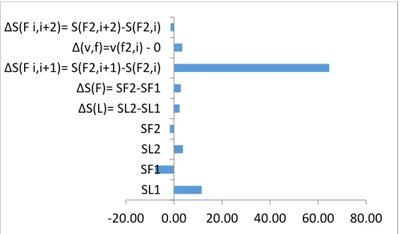
Figure 12. The Chart of Analyzing the Parameters Sensitivity based on the Behavioral Pattern of the Over Constant Reaction-Timid

3.2.3 Over Constant Reaction- Timid Driver

According to Figure 12, the results of analyzing the transmitted data sensitivity from nine parameters at the microscopic level indicates that three parameters of spacing difference of the follower vehicle while receiving the stop and congestion waves, spacing difference of the follower vehicle between two phases of deceleration and congestion and spacing of the leader vehicle when propagating the stop wave have the greatest effect on the amount of time between two phases, respectively.

3.2.3.1 The Artificial Neural Network

Parameters in the Microscopic Level

According to Figure 13, increasing the spacing difference between two phases of stop and congestion leads to decreasing the time of entering the stop leading to the congestion. Increasing the following spacing in the stop phase leads to increasing the maneuverability of the follower driver based on the over constant reaction- timid pattern. In other words, the follower driver is less likely to decelerate and increase the time between two phases due to providing the safe spacing. Increasing spacing in the congestion phase leads to decreasing the safe spacing. The follower driver has a tendency to faster slow down and reducing the time between two phases due to providing the safe headway in the congestion phase.

Figure 13. The Neural pattern of the time based on spacing difference of the follower vehicle between two stop and congestion phases

-40 -30 -20 -10 0 10 20 SL1

SF1 SL2 SF2 ΔS(L)= SL2-SL1 ΔS(F)= SF2-SF1 ΔS(F i,i+1)= S(F2,i+1)-S(F2,i) Δ(v,f)=v(f2,i) - 0 ΔS(F i,i+2)= S(F2,i+2)-S(F2,i)

0.00 10.00 20.00 30.00 40.00 50.00 60.00 70.00 80.00

-12.00 -10.00 -8.00 -6.00 -4.00 -2.00 0.00 2.00

Tim

e

(*

0.

1

, s

)

(14)

According to Figure 14, increasing the spacing difference between two deceleration and congestion phases leads to increasing the time for entering the stop leading up to the congestion. Similar to the behavioral pattern of the over reaction when the high safety of spacing at the time of propagating the deceleration wave leading up to the congestion enters the traffic oscillation, the follower driver based on the over constant reaction tends to a more deceleration, decreasing the time between two phases, due to

keeping the safe spacing fixed in order to increase his/her maneuverability in the traffic oscillation. According to Figure 15, increasing the spacing of the leader vehicle at the time of propagating the stop wave leads to decreasing the time between two phases. Although increasing spacing leads to flow traffic and increase the maneuverability of the follower driver based on the over constant reaction pattern, the driver tends to increase the deceleration, decreases the time between two phases, in order to increase and keep safe spacing

Figure 14. The neural pattern of time based on spacing difference of the follower vehicle between two deceleration and congestion phases

.

Figure 15. Spacing of the leader vehicle at propagating the stop wave

0.00 10.00 20.00 30.00 40.00 50.00 60.00 70.00 80.00

-200.00 -150.00 -100.00 -50.00 0.00

Tim

e

(*

0.

1

,

s)

Spacing (ft)

0.00 10.00 20.00 30.00 40.00 50.00 60.00 70.00 80.00 90.00

0.00 10.00 20.00 30.00 40.00 50.00

Tim

e

(*

0.

1

,

s)

(15)

4. Conclusion

Different behavioral reactions of the vehicle drivers in the traffic oscillation to the shock wave, received from the downstream, leads to the complexity of the stop-go traffic analysis. In this paper, the data trajectory of the vehicle platoon in the deceleration phase of the stop-go traffic was divided into three phases of deceleration wave, entry into the stop and congestion. The behavioral patterns of the follower driver in the vehicle platoon were identified and the parameters of each behavioral pattern were segregated at the microscopic level. Then, by applying neural network patterns, the effective parameters, at the microscopic level, on the time of entering the stop leads to the congestion based on each behavioral pattern had been analyzed. Due to lack of data, only the effective parameters of three behavioral patterns including: under reaction-timid, over-reaction-timid and the behavioral pattern with over constant reaction-timid at microscopic level were analyzed in the stop-go traffic. The results indicated that based on the behavioral pattern with under reaction-timid, the spacing difference of the follower vehicle between two phases of stop and congestion when receiving the wave and based on the behavioral pattern with overreaction-timid, spacing difference parameter of the follower vehicle between two phases of the deceleration and congestion and based on the behavioral pattern of the over constant reaction-timid, the spacing parameter of the leader vehicle at the time of propagating the wave are the most effective parameters on the dependent variable of time for entering the stop, at the microscopic level. According to table 4, based on the behavioral pattern with under reaction-timid,

increasing the spacing difference of the follower vehicle between two phases of stop and congestion leads to decreasing the stopping time leading up to the congestion. Increasing the follower spacing at the time of receiving the stop wave leads to decreasing the spacing difference between two phases. The follower driver based on the behavioral pattern with under reaction leads to decrease the safe spacing due to neglecting the received wave and reluctance to reduce spacing. In order to provide a safe spacing, it is necessary to increase the deceleration and decrease the time between two phases of stop and congestion. In other words, increasing the spacing of the follower driver when receiving the deceleration wave based on the behavioral pattern with overreaction increases the deceleration due to the keeping the safe spacing. Based on the behavioral pattern with overreaction-timid, increasing spacing difference of the follower vehicle between two phases of the deceleration and congestion leads to increasing the time between two phases. Increasing the spacing when receiving the deceleration wave leads to decreasing the spacing difference between two phases. The follower driver increases the deceleration at the time of receiving the wave due to keeping the safe spacing, which leads to decrease the stopping time between two phases. Based on the behavioral pattern of the over constant reaction, increasing the spacing of the leader vehicle at the time of propagating the wave leads to decrease the time between two phases. Although increasing the spacing of the leader vehicle leads to higher level of service for the traffic, but the follower driver, in order to keep the higher safe spacing, provides a more severe deceleration in the traffic oscillation.

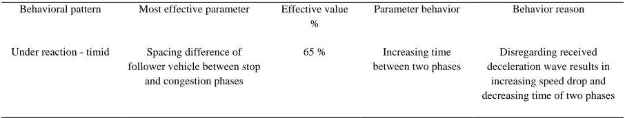
Table 4. The Time for Entering the Stop Leading to the Congestion

Behavior reason Parameter behavior

Effective value % Most effective parameter

Behavioral pattern

Disregarding received deceleration wave results in

increasing speed drop and decreasing time of two phases Increasing time

between two phases 65 %

Spacing difference of follower vehicle between stop

(16)

Increasing speed drop because of create constant enough safe spacing in traffic oscillation Increasing time

Spacing difference of follower vehicle between deceleration and congestion

phases Over reaction - timid

Creating enough safe spacing results in increasing speed drop and decreeing stop time Decreasing time

Leader spacing in propagation wave

Over constant reaction - timid

5. References

-Ahn, S. and Cassidy, M. (2006) “ Freeway traffic oscillations and vehicle lane-changemanoeuvres. In: Heydecker, B., Bell, M., Allsop, R. (Eds.)”, Forthcoming in 17thInternational Symposium on Transportation and Traffic Theory. Elsevier, NewYork.

-Ahn, S., Vadlamani, S. and Laval, J. A. (2011) “A method to account for non-steady state conditions in measuring traffic hysteresis." Transportation Research Part C: Emerging Technologies Vol. 34, pp. 138-147”

-Abdi, A. and Salehikalam, A. (2016) “Analyzing deceleration time lead to congestion based on behavior patterns”, Modares Civil Engineering Journal - Volume 16, Special Issue, Winter 1395, pp. 91-102.

-Arab Moghadam, M., Pahlavani, P., Naseralavi, S. (2016) “Prediction of car following behavior based on the instantaneous reaction time using an ANFIS-CART based model”, International Journal of Transportation Engineering , Article 4, Volume 4, Issue 2, pp.. 109-126.

-Bilbao-Ubillos, J. (2008) “The costs of urban congestion: estimation of welfare losses arising from congestion on cross-town link roads”, Transportation Research Part A Vol. 42, No. 8, pp.1098–11082.

-Chen, D., Laval, J. A. Zheng, Z. and Ahn, S. (2012a) “Traffic oscillations: a behavioral car-following model”, Transportation Research Part B, Vol. 46, No. 6, pp. 744-761.

-Chen, D., Laval, J. A., Ahn, S. and Zheng, Z. (2012b) “Microscopic traffic hysteresis in traffic oscillations: A behavioral pespective”, Transportation Research Part B, Vol.43 A. pp.126-141.

-Del Castillo, J. M. (2001) “Propagation of perturbations in dense traffic flow: a model and its implications”, Transportation Research Part B Vol. 35, pp. 367-389.

-Edie, L. C. and Baverez, E. (1967) “Generation and propagation of stop-start traffic waves”, Proceedings of Third International Symposium on the Theory of Traffic Flow. American Elsevier Publishing Co. New York. pp. 26-37.

-Forbes, T. W., Zagorski, H.J. Holshouser, E. L. and Deterline, W. A. (1958) “Measurement of driver reactions to tunnel conditions”, Proceedings of Highway Research Board.Vol.37, pp. 345-357.

-Herman, R. and Potts, R. B. (1961) “Single-lane traffic theory and experiment”, Proceedings of Symposium on the Theory of Traffic Flow (R. Herman Ed.). Elsevier publishing Co. Amsterdam. pp. 120-146.

-Herman, R. and Rothery, R. (1967) “Propagation of disturbances in vehicular platoons”, Proceedings of Third International Symposium on the Theory of Traffic Flow (L.C. Edie, Ed.), American Elsevier publishing Co. New York. pp. 26-37.

(17)

399 International Journal of Transportation Engineering, Vol.5/ No.4/ Spring 2018 the IEEE Intelligent Transportation System, Vol.

1, China, pp. 346–351.

-Kim, T. and Zhang, H. M. (2004) “Gap time and stochastic wave propagation”, IEEE Intelligent Transportation Systems Conference, pp. 88-93.

-Koshi, M., Kuwahara, M. and Akahane, H. (1992) “Capacity of sags and tunnels injapanese motorways”, ITE Journal (May issue), pp.17–29.

-Karlaftis, M. G. and Vlahogianni, E. I. (2011) “Statistics versus neural networks in transportation research: Differences, similarities and some insights”, Transportation Research Part C: Emerging Technologies. Vol. 19, No. 3, pp. 387-399.

-Khodayari, A. and Ghaffari, A. (2011) “ Modify car following model human effects based on locally linear neuro fuzzy”, Intelligent Vehicles Symposium (IV), 2011 IEEE. pp. 661-666.

-Laval, J. A. and Daganzo, C. F. (2006) “Lane-changing in traffic streams”, Transportation Research Part B Vol. 40, No. 3, pp. 251–264.

-Laval, J. A. (2006) “Stochastic processes of moving bottlenecks: Approximate formulas for highway capacity”, Transportation Research Record, pp. 86–91.

-Laval, J. A. and Leclercq, L. (2010) “A mechanism to describe the formation and propagation of stop-and-go waves in congested freeway traffic”, Philosophical Transactions of The Royal Society A. 368, pp. 4519-4541.

-Laval A. J. (2010) “Hysteresis in traffic flow revisited: An improved measurement method, Transportation Research”, Part B. Vol. 45, No 2, pp. 385–391.

-Laval A. J. (2009) “Hysteresis in the fundamental diagram: impact of measurement methods”, 89th Annual Meeting of the Transportation Research Board, Washington, D.C.

-Mauch, M. and Cassidy, M. J. (2002) “Freeway traffic oscillations: observation and predictions”, The 15th International Symposium on Transportation and Traffic flow Theory.

-Newell, G. F. (1962) “Theories of instability in dense highway traffic”, Journal of the Operations Research Society of Japan Vol. 5, pp.9–54.

-Newell, G. F. (2002) “A simplified car-following theory: a lower order model”, Transportation Research Part B Vol. 36, pp. 196-205.

-NGSIM. Accessed at: http://ngsim-community.org/

-Orfanou, F., Vlahogianni, E and Karlaftis, M. (2012) “Identifying features of traffic hystersis on freeways, Transportation Research, Part B.

-Panwai, S. and Dia, H. (2007) “ Neural agent car-following models, IEEE Transactions on Intelligent Transportation Systems,Vol. 8, No. 1, pp. 60–70.

-Trajectory Explorer. Accessed at: http://trafficlab.ce.gatech.edu/tools.html.

-Treiterer, J. and Myer, J. A (1974) “The hysteresis phenomenon in traffic flow”, Proceedings of the Sixth Symposium on Transportation and Traffic Flow Theory. D. J. Buckley (Ed.). pp. 213-219.

-Xiaoliang, Ma. (2006) “A neural – fuzzy framework for modeling car following behavior”, Systems, Man and Cybernetics, 2006. SMC'06. IEEE International Conference on. Vol. 2. IEEE, 2006, pp. 770-776.

(18)

-Zheng, Z., Ahn, S., Chen, D. and Laval, J. A. (2011) “Freeway traffic oscillations: Microscopic analysis of formations and propagations using wavelet transform”, Transportation Research Part B, Vol. 45, No. 9, pp. 1378-1388.

-Zheng, Z., Ahn, S., Chen, D. and Laval, J. (2011a) “Applications of wavelet transform for analysis of freeway traffic: bottlenecks, transient traffic, and traffic oscillations. Transportation Research Part B Vol. 45 No. 2, pp.372–384.

-Zheng, Z., Ahn, S., Chen, D., Laval, J.A. (2011b) “Freeway traffic oscillations: microscopic analysis of formations and propagations using wavelet transform”. The 19th

International Symposium on Transportation and Traffic flow Theory, pp.717–731.

-Zhang, H. M. (1999) “A mathematical theory of traffic hysteresis”, Transportation Research Part B, Vol. 33, pp. 1-23.

-Zhang, H. M. and Kim, T. (2005) “A car-following theory for multiphase vehicular traffic flow”, Transportation Research Part B, Vol. 39, pp. 385-399.