Int. J. Data Envelopment Analysis (ISSN 2345-458X)
Vol.5, No.1, Year 2017 Article ID IJDEA-00422, 10 pages Research Article
Sensitivity in ranking for perturbations of data
in DEA
P. Zamani
*Faculty of Engineering, Qom Branch, Islamic Azad University, Qom, Iran
Received September 19, 2016, Accepted December 23, 2106 Abstract
Sensitivity analysis in Data Envelopment Analysis (DEA) is studied for perturbations of data for which ranking of efficient Decision Making Units (DMUs) is preserved. Sufficient conditions for efficient DMUs to preserve their ranks under the perturbations of data are achieved. Accordingly, it can be found out how to change outputs or inputs of an efficient DMU while preserving ranking of all efficient DMUs. In addition, an illustrative numerical example is provided to receive a better comprehension.
Keywords: Data Envelopment Analysis, Ranking, Sensitivity Analysis.
*. Email address: [email protected]
1. Introduction
Data envelopment analysis (DEA) is a mathematical programming technique to evaluate relative efficiency of decision making units (DMUs) with multiple input-output. It computes a scalar measure of efficiency and discriminates between efficient and inefficient DMUs. Hence, it ranks DMUs unless some DMUs have efficiency score unity. One of the interesting research subjects is to discriminate among efficient DMUs. Several authors proposed methods for ranking the best performers (see [2, 9, 10, 13, 14 and 16] among others).
Another feature of this DEA technique which has been studied by many researchers is sensitivity analysis. One of the topics of DEA sensitivity analysis is based upon data variations. The first DEA sensitivity analysis paper by Charnes et al. [5] examined a change in a single output. This was followed by a series of sensitivity analysis articles by Charnes and Neralic [7] to allow simultaneous proportional changes of all inputs and outputs for a specific DMU which is under consideration. This data variation condition is relaxed in Zhu [15] and Seiford and Zhu [12] to a situation where inputs or outputs can be changed individually. The DEA sensitivity analysis methods, we have just reviewed, are all developed for the situation where data variations are only applied to the under evaluation efficient DMU, and the data for the other remaining DMUs are assumed fixed.
Seiford and Zhu [11] generalized the technique in Zhu [15] and Seiford and Zhu [12] to the worst-case scenario where the efficiency of the under evaluation DMU is deteriorating while the efficiencies of the other DMUs are improving. The mentioned sensitivity analysis methods are based on the increase of some or all inputs and the decrease of some or all the outputs. In this paper, the attention is devoted to the case where the decrease of outputs and the
increase of inputs for an efficient DMUp are not preformed simultaneously.
The purpose of this research is to study sensitivity analysis in DEA for the case of perturbations of outputs or of inputs of an efficient DMU preserving ranking of all efficient DMUs. In that way sufficient conditions for efficient DMUs to preserve their ranks under the perturbations of data (inputs or outputs) are provided. Furthermore, an illustrative example is provided.
The paper is organized as follows: Section 2 briefly reviews a mathematical basis used for this study. Sensitivity analysis in LP under different problem variations is discussed in section 3. In section 4, sensitivity analysis in DEA for the case of changes of data is studied. In particular, the way of changing outputs of an efficient DMU while preserving ranking of all efficient DMUs is represented. In section 5, an illustrative example is given. Concluding remarks are summarized in the last section. 2. Background
Suppose that we have a set of n DMUs each of which utilizes m inputs to produce s outputs. The inputs and outputs for all of the DMUs are assumed to be nonnegative, but at least one component of every input and output vector is positive.
For evaluating the efficiency of DMUp
(p 1,...,n ), we can use the envelopment forms of (the input-oriented) CCR and BCC model.
(1a): Input-oriented CCR model Min
s.t j p
n
j
j
x
x
1
j p n
j
j
y
y
1
n
j
j
0
,
1
,...,
(1b): Input-oriented BCC model (1)
s.t j p n
j
j
x
x
1
j p n
j
j
y
y
1
n
j j 1
1
n
j
j
0
,
1
,...,
For an inefficient DMUj, we define its reference set
E
j by :
* 0
1, ..., (1) ((1 ) (1 ))
p p in some optimal
E n
j
Solution of a or b
Definition 1. DMUp (p{1,...,n}) is CCR efficient (BCC efficient), if and only if
1
*
in (1a) ((1b)) and the optimal value of (2 a) ((2 b)) is equal to zero:(2 a):Max es es s.t
n
j
p j
j
x
s
x
1
n
j
p j
j
y
s
y
1
n
j
j
0
,
1
,...,
0 ,
0
s
s
(2 b): Max es es (2) s.t
n
j
p j
j
x
s
x
1
n
j
p j
j
y
s
y
1
n
j j 1
1
n
j
j
0
,
1
,...,
0 ,
0
s
s
The efficiency score obtained by standard DEA models cannot be used for ranking efficient DMUs. So Charnes et al. [4] proposed a procedure for ranking efficient
DMUs by simply counting the number of times they appear in the reference sets of inefficient units. Therefore, an efficient unit is highly ranked if it is chosen as a useful reference by many other inefficient units. 3. Sensitivity analysis in LP
When the final optimal solution of an LP has been obtained, we may discover that some of the entries in the cost coefficients, right-hand-side constants or constraint matrix have to be changed or that extra constraints or variables have to be introduced into the model. It is important to be able to find the new optimal solution of the problem without the expensive task of resolving the problem from scratch. These and other related topics constitute sensitivity analysis. Some methods for updating the optimal solution under different problem variations will be briefly discussed.
3.1. Change in the cost coefficient
Suppose that the cost coefficient of one of the variables is changed. The effect of this change on the final tableau will occur in the cost row. That means dual feasibility may be lost.
3.2. Change in the right-hand-side
In this case, primal optimality is maintained. The only possible violation of optimality is that the new right-hand-side vector may have some negative entries; therefore, the dual simplex algorithm should be applied until a new terminal basis is obtained.
change may destroy one or both primal and dual feasibility.
3.4. Introducing a new activity
Suppose a new activity has to be introduced into the model. If the optimality condition for the new variable is satisfied, the value of this variable in optimality will vanish and the current solution will remain optimal. Otherwise, the simplex method continues to find the new optimal solution.
3.5. Introducing a new constraint
Suppose that a new constraint is added to the problem. This operation is dual to that adding a new activity. If the optimal solution of the original problem satisfies the added constraint, it is obvious that the point will be also an optimal solution of the new problem. If, on the other hand, the point does not satisfy the new constraint, the dual simplex method can be used to find the new optimal solution.
4. Nonnegative perturbations of data In this section, we are interested in particular variations of outputs of an efficient DMU that preserves the ranking of all efficient DMUs. In addition, Variations of inputs are alike.
For this purpose, we first find all efficient DMUs and reference sets of inefficient DMUs (with models (1) and (2)). By using the Charnes ranking method, we obtain the ranks of all efficient DMUs.
Now, we consider decrease of outputs of an efficient DMUp:
s r
y
yˆrp rp r 0,r 0, 1,..., (3)
We note that by decreasing the outputs of an efficient DMUp, the new efficient frontier gets closer to the inefficient DMUs (even changing some of these inefficient DMUs to efficient), that is, the ranking results of efficient DMUs obtained by Charnes may be affected by this perturbation.
Let
J
p
{
j
1,...,
j
l}
be the set of indices associated with the inefficient DMUs in whicht
j
E
p
(t=1,…,l). The region of variations of
(
(
1,...,
s))for whichJ
premains unchanged is a region within which the ranking of efficient DMUs is preserved. In other words, we want to preserve the inefficiency of all inefficient DMUs in a region, keeping the reference sets for them the same.From the definition of the reference set, for each inefficient DMUj
t(t=1,…,l) vector
t p p
y
x
,
)
(
must occur in every optimal basis of (1).t
j
E
p
for each t=1,…,l as long as all optimum bases corresponding to these inefficient DMUs include
*pas basic variable.Let
B
is an optimal basis for (1) in evaluating an inefficient DMUjt(t=1,…,l) (
It is important to note that the perturbations of outputs (3) do not affect the right hand side of this linear programming problem). Now we attempt to identify a region within whichB remains an optimal basis.
Perturbations (3) are accompanied by alteration in the inverse of the optimal basis matrix(B1). From the discussion in section (3.3) this change may destroy either or both primal and dual feasibility. We therefore proceed to show how these variations can be accommodated by building on the inverse which is already available in the optimum simplex tableau. Recall that the vector
(
x
p,
y
p)
tmust occur in every optimal basis of (1) in evaluating DMUjt(t=1,…,l). To perturb the
* p
. Let Bˆ BT denote the altered basisWhere
pth column pth column 0 0 0 0 0 0 0 0 0 0 1 s T ( 0 0 0 0 0 0 0 0 0 0 0 0 0 1 s T
) (4)
In order to get the perturbed basis inverse, we can use the Sherman-Morrison-Woodbury formula (see, for example, [8, p. 11]).
1 1
1 1 1 1 1
ˆ
( ) ( )
( )
B B T
B B T I B T B
(5)
Using the abbreviation 1 1
)
(
T I B T
R (6)
We can write (5) as 1 1 1 1
)
ˆ
(
B
B
B
RB
(7) Theorem 1: For each efficient DMUp, let}
,...,
{
1 lp
j
j
J
be the set of indices associated with the inefficient DMUs in whicht
j
E
p
(t=1,…,l). SupposeBis an optimal basis for (1) in evaluating an inefficient DMUjt(t=1,…,l). Sufficient
conditions for efficient DMUs to preserve their ranks under the perturbations (3) are
n
j
wRy
c
z
j
j
j,
1
,...,
(8)j an index of nonbasic variables
0 )
(IB1R B1b (9)
Where
y
j
B
1a
j and wcBB1in which the components ofc
Bare the coefficients in the objective function corresponding to the basic variable.Proof. We can characterize optimality of the perturbed basis Bˆ BT from the conditions that all nonbasic variables must continue to price out unfavorably, and all basic variables be non-negative. That is respectively:
Case I:
(
z
ˆ
j
c
j)
0
, j 1,...,n With zj cB B 1aj) ˆ (
ˆ
Using notation (7) we have j j B
j
j
c
c
B
B
RB
a
c
z
ˆ
(
1
1 1)
,j1,...,nj j B
j
B
B
a
c
B
RB
a
c
c
1 1 1j B
j j
B
B
a
c
c
B
RB
a
c
1
1 1
0
z
jc
jwRy
jThe last expression can be written in an equivalent form
z
j
c
j
wRy
j, j1,...,n. Case II:1 1 1 1
1 1 1 1 1
ˆ
0 ( ) ( )
( )
B b B B RB b
B b B RB b I B R B b
It means that (I B1R)B1b0and this completes the proof.
For each inefficient DMUj
t, the conditions
of Theorem 1 will determine a region within which the corresponding optimum basis remains optimal. In other words, under these conditions, p remains a member of the reference set of each inefficient DMUj
t(t=1,…,l), so the ranking of efficient
DMUs is preserved. Overall assurance region is defined as the intersection of all regions in which the conditions of Theorem 1 are maintained. It should be noted that there may be alternative optimal solutions for (1), so we need to deal with any one optimal bases satisfying the conditions of Theorem 1.
5. Numerical example
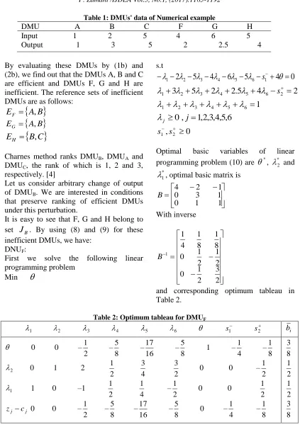
Table 1: DMUs' data of Numerical example
DMU A B C F G H Input 1 2 5 4 6 5
Output 1 3 5 2 2.5 4 By evaluating these DMUs by (1b) and
(2b), we find out that the DMUs A, B and C are efficient and DMUs F, G and H are inefficient. The reference sets of inefficient DMUs are as follows:
A
B
E
F
,
A B EG ,
B
C
E
H
,
Charnes method ranks DMUB, DMUA and DMUC, the rank of which is 1, 2 and 3, respectively. [4]
Let us consider arbitrary change of output of DMUB. We are interested in conditions that preserve ranking of efficient DMUs under this perturbation.
It is easy to see that F, G and H belong to set
J
B. By using (8) and (9) for these inefficient DMUs, we have:DNUF:
First we solve the following linear programming problem
Min
s.t
0
4
5
6
4
5
2
2 3 4 5 6 11
s
2
4
5
.
2
2
5
3
2 3 4 5 6 21
s
1
6 5 4 3 21
6
,
5
,
4
,
3
,
2
,
1
,
0
j
j
0 , 2 1 s sOptimal basic variables of linear programming problem (10) are
*,
*2 and* 1
, optimal basic matrix is 1 1 0 1 3 0 1 2 4 B With inverse 2 3 2 1 0 2 1 2 1 0 8 1 8 1 4 1 1 B
and corresponding optimum tableau in Table 2.
Table 2: Optimum tableau for DMUF
1 2 3 4 5 6 1
s s2 bi
0 0 – 2 1 – 8 5 – 16 17 – 8 5
1 – 4 1 – 8 1 2
0 1 2 2 1 4 3 2 3
0 0 – 2 1
1
1 0 –1 2 1 4 1 – 2 1
0 0 2 1
j j c
z 0 0 – 2 1 – 8 5 – 16 17 – 8 5
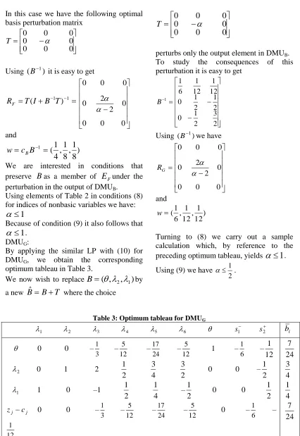
In this case we have the following optimal basis perturbation matrix
0 0 0 0 0 0 0 0 T
Using (B1) it is easy to get
1 1
)
(I B T
T RF 0 0 0 0 2 2 0 0 0 0 and ) 8 1 , 8 1 , 4 1 ( 1 B c w B
We are interested in conditions that preserve
B
as a member ofE
Funder the perturbation in the output of DMUB.Using elements of Table 2 in conditions (8) for indices of nonbasic variables we have:
1
Because of condition (9) it also follows that
1
.DMUG:
By applying the similar LP with (10) for DMUG, we obtain the corresponding optimum tableau in Table 3.
We now wish to replace
B
(
,
2,
1)
by a new Bˆ BT where the choice 0 0 0 0 0 0 0 0
Tperturbs only the output element in DMUB. To study the consequences of this perturbation it is easy to get
2 3 2 1 0 2 1 2 1 0 12 1 12 1 6 1 1 B
Using (B1)we have
0 0 0 0 2 2 0 0 0 0 G R and ) 12 1 , 12 1 , 6 1 ( w
Turning to (8) we carry out a sample calculation which, by reference to the preceding optimum tableau, yields
1
. Using (9) we have2 1
.
Table 3: Optimum tableau for DMUG
1 2 3 4 5 6 1
s s2 bi 0 0 –
3 1 – 12 5 – 24 17 – 12 5
1 – 6 1
– 12
1
2 0 1 2 2 1 4 3 2 3
0 0 – 2 1
1 1 0 –1 2 1 4 1 – 2 1
0 0 2 1
j j c
z 0 0 – 3 1 – 12 5 – 24 17 – 12 5
Table 4: Optimum tableau for DMUH
1 2 3 4 5 6 s1 s2 bi –
5 2
0 0 – 10 7 – 20 19 – 10 3
1 – 5 1
–
10 3
3 –1 0 1 – 2 1 – 4 1 2 1
0 0 – 2 1
2 2 1 0 2 3 4 5 2 1
0 0 2 1
j j c
z –
5 2
0 0 – 10 7 – 20 19 – 10 3
0 – 5 1 – 10 3 10 7 2 1 2 1 10 7
DNUH:
In the similar way for inefficient DMUH, we produce the full details of the optimum tableau as shown in table 4.
As can be seen, we have the following optimal basis matrix
1 1 0 3 5 0 2 5 5 ) , ,
(
3
2B With inverse 2 5 2 1 0 2 3 2 1 0 2 1 10 3 5 1 1 B
and the following change of the optimal basis matrix 0 0 0 0 0 0 0 0
ˆ B
B
Using (B1) it is easy to get
0 0 0 2 2 0 0 0 0 0 H R And ) 2 1 , 10 3 , 5 1 ( w
According to the conditions provided by (8), it follows that 21. Similarly we also obtain 1 from condition (9). Finally, from the intersection of all intervals,
must be in the range of]. 5 . 0 , 0
[ After the change of output of DMUB in this range, the ranking of efficient DMUs will be preserved.
6. Conclusion
References
[1] Adler, N., Friedman, L., Sinuany-Stern, Z. Review of ranking methods in data envelopment analysis context. European Journal of Operational Research. 2002; 140(2): 249–265.
[2] Andersen, P., Petersen, N. C. A procedure for ranking efficient units in data envelopment analysis. Management Science. 1993;39(10):1261-1264.
[3] Banker, R. D., Charnes, A., Cooper, W. W. Some models for estimating technical and scale inefficiencies in data envelopment analysis. Management Science. 1984;30(9): 1078-1092.
[4] Charnes, A., Clark, C. T., Cooper, W. W., Golany, B. A developmental study of data envelopment analysis in measuring the efficiency of maintenance units in the U.S. air forces. Annals of Operations Research. 1985; 2(1-4):95-112.
[5] Charnes, A., Cooper, W. W., Lewin, A. Y., Morey, R. C., Rousseau, J. Sensitivity and stability analysis in DEA. Annals of Operations Research. 1985; 2(1):139-156. [6] Charnes, A., Cooper, W. W., Rhodes, E. Measuring the efficiency of decision making units. European Journal of Operational Research. 1978;2(6):429-444. [7] Charnes, A., Neralic, L. Sensitivity analysis of the proportionate change of inputs (or outputs) in data envelopment analysis. Glasnik Matematicki. 1992; 27(2): 393-405.
[8] Golub, G. H., Van Loan, C. F. Matrix Computations. 4th edition. Baltimore, Maryland: Johns Hopkins University Press; 2013.
[9] Hibiki, N., Sueyoshi, T. DEA sensitivity analysis by changing a reference set: Regional contribution to Japanese industrial
development. Omega. 1999; 27(2): 139-153.
[10] Mehrabian, S., Alirezaee, M. R., Jahanshahloo, G. R. A complete efficiency ranking of decision making units in data envelopment analysis. Computational optimization and applications. 1999; 14(2): 261–266.
[11] Seiford, L. M., Zhu, J. Sensitivity analysis of DEA models for simultaneous changes in all the data. Journal of the Operational Research Society. 1998a; 49(10): 1060-1071.
[12] Seiford, L. M., Zhu, J. Stability regions for maintaining efficiency in data envelopment analysis. European Journal of Operational Research. 1998b; 108(1):127-139.
[13] Seiford, L. M., Zhu, J. Infeasibility of super efficiency data envelopment analysis models. INFOR. 1999; 37(2):174-187. [14] Sexton, T. R., Silkman, R. H., Hogan, A. J. Data envelopment analysis: Critique and extensions. New Directions for Program Evaluation. 1986; 1986(32):73-105.
[15] Zhu, J. Robustness of the efficient DMUs in data envelopment analysis. European Journal of Operational Research. 1996; 90(3):451-460.