Supply Chain Coordination using Different Modes of Transportation Considering Stochastic Price-Dependent Demand and Periodic Review Replenishment Policy

(1)

137 International Journal of Transportation Engineering, Vol. 5/ No. 2/ Autumn 2017

Supply Chain Coordination using Different Modes of

Transportation Considering Stochastic Price-Dependent

Demand and Periodic Review Replenishment Policy

Maryam Johari1, Seyyed-Mahdi Hosseini-Motlagh2, Mohammadreza Nematollahi3

Received: 12. 03. 2017 Accepted: 26. 04. 2017

Abstract

In this paper, an incentive scheme based on crashing lead time is proposed to coordinate a supplier-retailer supply chain (SC). In the investigated SC, the supplier applies a lot-for-lot replenishment policy to replenish its stock and determines the replenishment multiplier. Moreover, the transportation lead time is considered under the control of the supplier. The retailer as downstream member manages his inventory system according to the periodic review replenishment system (R, T). The review period (T) and order-up-to level (R) decisions along with the retail price are simultaneously optimized by the retailer. These decisions are made by the retailer influence the profitability of SC as well as the supplier's profitability. The investigated SC is modeled under three different decision making structures, i.e., (1) decentralized decision making model, (2) centralized decision making model, and (3) coordinated decision making model. By developing a lead time reduction policy as an incentive strategy, the pricing and periodic review replenishment decisions are coordinated. In the proposed incentive approach, the supplier by spending more cost and changing a fast transportation mode aims to crash the lead time in order to entice the retailer to accept the joint decision making strategy. In the suggested incentive scheme, two transportation modes (one slow and one fast) are supposed. Further, maximum and minimum lead time reduction, which are acceptable for both members, are determined. Moreover, a set of numerical examples along with a real case are carried out to demonstrate the performance and applicability of the developed models. The results demonstrate that the proposed incentive strategy is able to achieve channel coordination. Moreover, the results show the applicability of the developed coordination model under the high demand uncertainty. In addition, the proposed coordination model will fairly share the obtained profits between two SC members.

Keywords: Transportation mode selection, lead time reduction, supply chain coordination, pricing, periodic review inventory system.

Corresponding author Email: [email protected]

(2)

Supply Chain Coordination Using Different Modes of Transportation Considering Stochastic …

International Journal of Transportation Engineering, 138 Vol. 5/ No. 2/ Autumn 2017

1. Introduction

The selection of the proper transportation mode can be considered as a substantial decision in the supply chain management (SCM) including the trade-off between SC costs and customer service level [Rushton et al. 2010]. Various transportation modes result in different lead time (delivery time) and cost for SC members and consequently it is of high importance to optimize decisions regarding shipping modes. The two common transportation modes: full truckload (FTL) and less than truckload (LTL) make significant costs for both shipper and buyer as well as different lead time. Under FTL transportation mode, the items take the total space of the truck. Although FTL mode delivers the items to the buyer with low lead time and reduces inventory cost, it imposes more transportation cost for the shipper. On the other hand, in LTL transportation mode, the shipper just pay the amount of used space on the carrier's truck. In other words, the loads may not occupy the whole accessible space of the truck. In addition, the rest space could be shared with other shippers which may occur many stops which in turn leads to high lead time for the buyer. Thus, LTL mode increases lead time toward FTL mode. As a result, selecting slow mode reduces cost for the supplier but the retailer receives the goods with high lead time which in turn needs to stock more and spend high inventory cost. While fast mode delivers items to the retailer in low lead time along with decreasing the inventory cost for the retailer but enhances the supplier's transportation cost. Therefore, regarding to lead time, decisions may create conflicts among supply chain members. According to Leng and Parlar [Leng and Parlar, 2009], crashing lead time can lead to smaller safety stocks, smaller shortage items, and a decrease in the bull whip effect in addition to lower costs. Thus, controlling lead time in the supply chain could be of mutually beneficial for the SC members. In general, decisions which are made by one SC member greatly influence the SC profitability as well as other SC members. Coordinated decision making model can motivate

the SC members to change the locally optimal decisions, which create the sub-optimal performance, to globally optimal decisions, which are made based on the entire SC stand point [Sinha and Sarmah, 2010]. There are various mechanisms used to coordinate the SC decisions such as quantity discount contract [Chaharsooghi, Heydari, and Kamalabadi, 2011], delay in payments contract [Heydari, 2015], revenue sharing contract [Arani Vafa, Rabbani, and Rafiei, 2016], buy back contract [Ai et al., 2012] and so forth. In the SCM literature, coordinated scheme have been extensively studied by many scholars to coordinate the essential decisions in the supply chain such as social responsibility [Nematollahi, Hosseini-Motlagh, and Heydari, 2017a], lead time [Heydari and Norouzinasab, 2016], safety stock and reorder point [Heydari, 2014a; Chaharsooghi and Heydari, 2010a], and inventory [Sajadieh and Akbari Jokar, 2009]. Besides, Pricing is one of the crucial decisions in the supply chain management that requires to be coordinated. Coordination of pricing decision could be of high importance to solve the double marginalization and increase the SC profitability [Mokhlesian et al., 2015]. Although many researches have considered joint pricing and inventory replenishment coordination in a supply chain, these studies have investigated the coordination of pricing and continuous replenishment decisions. In other words, the simultaneous coordination of pricing and periodic review inventory systems was not considered previously. In addition, there have been handful researches on the coordination of periodic review inventory policies such as [Nematollahi, Hosseini-Motlagh, and Heydari, 2017b; Johari, Hosseini-Motlagh, and Nematollahi, 2017; Hojati et al. 2017].

(3)

Maryam Johari, Seyyed-Mahdi Hosseini-Motlagh, Mohammadreza Nematollahi

decisions in a two echelon SC including one supplier and one retailer. In the proposed SC model, the supplier manages his inventory system based on a lot-for-lot replenishment policy and decides on the replenishment multiplier. Further, the transportation lead time is considered to be deterministic. On the other hand, the retailer exerts the periodic review inventory system (R, T) where both the review period (T) and order-up-to-level (R) are retailer's decision variables along with the retail price. Moreover, the retailer faces a stochastic price dependent demand following a normal distribution. Furthermore, if the customer’s demand is not met instantly the demand will be lost partially. The pricing and replenishment decisions are made by the retailer impact on both the profitability of the supplier and the entire SC. Indeed, retailer’s order-up-to-level impacts safety stock, service level, and amount of lost sales at the retailer’s site which in turn affects the sales of SC besides profitability of the SC as well as profitability of the supplier. In addition, under a price dependent demand individually decisions on the retail price could influence the market demand which in turn affect the profitability of the supplier and SC profitability. The investigated SC is modeled under three different structures: (1) decentralized decision making structure, (2) centralized decision making structure, and (3) coordinated decision making structure. Under the decentralized structure, each SC member seeks to maximize its profit function without considering the other SC member. It is obvious that these individually decisions are made by each SC member are not optimal from the entire SC perspective. Under the centralized structure, all SC decisions are made from the whole SC point of view. Although the centralized solution makes more profit for the entire SC, this joint decision making may incur losses for the retailer. Thus, the retailer will not accept the joint decision making. As a result, we suggest a coordination plan through lead time reduction as an incentive strategy to ensure the

profitability of both SC members. Similar to the work of Heydari, Zaabi-Ahmadi, and Choi [Heydari, Zaabi-Ahmadi, and Choi, 2016] in the developed incentive scheme, the supplier aims to reduce the transportation lead time by spending more cost and also improving the transportation mode to convince the retailer to shift the locally decision making toward the joint decision making. Our proposed coordination plan is capable of enhancing the profitability of both SC members along with sharing the extra benefits between two SC members fairly. The main contribution of our investigation to the current literature is the coordinating pricing and periodic review replenishment decisions through transportation lead time crashing as an incentive approach.

The rest of the paper is organized as follows. Next section provides the literature review on the lead time reduction in addition to the supply chain coordination under the inventory and pricing decisions. The notations and assumptions are made in Section 3. Section 4 presents the SC model under three different decision making structures and optimal solution algorithms. Further, numerical experiments along with a real case are carried out in section 5. Finally, section 6 concludes the paper and discusses future research directions.

2. Literature Review

(4)

production time, and shipping time. Moreover, they examined the issue of determining the responsible for the shipping lead time. Further, Chaharsooghi and Heydari [Chaharsooghi and Heydari, 2010b] analyzed the impacts of both lead time mean and lead time variance reduction on the supply chain performance. Their simulation models indicated that LT variance has a stronger effect on SC performance measures such as bullwhip effect, the number of stock-outs, and holding inventory. Arkan and Hejazi [Arkan and Hejazi, 2012] later designed the supply chain coordination in a two level SC through delay in payments under controllable lead time and ordering cost. Moreover, Li et al. [Li et al., 2012] formulated a coordination model under full information sharing and private information to examine the effects of crashing lead time on the inventory cost. In their model, the lead time reduction was assumed to be under the control of the buyers. Afterwards, Heydari [Heydari, 2014b] developed a coordination model using lead time uncertainty crashing to coordinate the service level in a supplier-retailer chain. The lead time variability was considered to be under the control of the supplier. In spite of the most studies in the related literature, he considered the lead time was stochastic. In another research, Heydari, Ahmadi, and Choi [Heydari, Zaabi-Ahmadi, and Choi, 2016] proposed a coordination model through shipping lead time reduction in a seller-buyer chain. They exploited two shipping modes (fast and slow) in their investigated model. The seller by spending more cost along with switching a fast shipping mode reduced the lead time. They proposed a fixed-charge step function to calculate the lead time crashing cost. Coordinating joint pricing and inventory decisions has broadly addressed in the SC coordination literature to improve the SC profitability. Cohen [Cohen, 1977] was the first researcher who developed the optimal joint pricing and inventory decisions. Boyacı and Gallego [Boyacı and Gallego, 2002] later

(5)

wholesale price contract to coordinate the SC decisions.

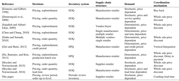
According to the previous literature most researches on the supply chain coordination using lead time crashing have investigated EOQ inventory policy. However, periodic review replenishment system is important as well. In addition, according to Table 1, none of the papers have aimed to coordinate the pricing decisions through lead time crashing scheme. To extend the application of lead time reduction scheme in real-world cases, a transportation lead time crashing as an incentive mechanism is proposed to coordinate joint pricing and periodic review inventory decisions. Through the proposed incentive mechanism, the supplier aims to reduce the transportation lead time by spending more cost and also enhancing the transportation mode to convince the retailer to change the locally decision making toward the joint decision making. Further, two transportation modes (one slow and one fast) are incorporated into the suggested incentive scheme. In our investigation, the supplier exerts a certain transportation mode for a specific lead time reduction and for more crashing lead time improves the transportation mode by switching to fast mode. To create a realistic model, in our proposed incentive scheme, the lead time crashing cost is considered.

3. Notations and Assumptions

The following notations and assumptions are used throughout this paper.

3.1 Notations

The notations applied in this paper are as follows.

Decision variables

T : Review period duration R : Order-up-to-level pr : Retail price

n : Supplier's replenishment multiplier (integral number of shipments to retailer)

Parameters

D(p_r) : Expected demand rate per year at retail price pr

𝒶 : Market size

Ɓ : Price-elasticity coefficient of demand ℓ : Lead time duration

X+_{: Maximum value of x and 0, that is}_X+₌ max {x, 0}

X : Protection interval (T + ℓ) demand that has a normal distribution function with finite mean D(T + ℓ) and standard deviation 𝜉√T + ℓ 𝜉 ∶ Standard deviation of the demand per unit time Ar: Retailer's fixed ordering cost per order h_r: Retailer's inventory holding cost per item per year w : Wholesale price

e : Purchase cost of the supplier per item As: Supplier’s fixed ordering cost per order h_s: Supplier’s average inventory holding cost per item per year

π : Shortage cost per item short

θ∶ Proportion of the demand during the stock-out period that will be lost, 0 < θ < 1

ω : Bargaining power of retailer

CR_SL: Cost of each percent of lead time reduction in slow transportation mode

CR_F: Cost of each percent of lead time reduction in fast transportation mode

F : Point at which more lead time reduction requires shifting to the enhanced (fast) transportation mode

M : Maximum possible lead time crashing C : Fixed cost for shifting from slow to fast transportation mode

LTR : Percentage of lead time reduction

(6)

Table 1. Comparing previous related works and this paper

Reference Decisions Inventory system Supply chain

structure Demand

Coordination mechanism

[Emmons and Gilbert,

1998] Pricing, replenishment EOQ Manufacturer-retailer

Stochastic, price

dependent Buy back

[Dumrongsiri et al.,

2008] Pricing, order quantity EOQ Manufacturer-retailer

Stochastic, price and service quality dependent

Whole sale price discount

[Sajadieh and

Akbari-Jokar, 2009] Pricing, replenishment EOQ Vendor-buyer

Deterministic, price dependent

[Chen and Chang, 2010] Pricing, replenishment EOQ Single manufacturer-multiple retailer

Deterministic, price and time dependent [Sinha and Sarmah,

2010] Pricing, order quantity EOQ

Multiple vendors-single retailer

[Giri and Maiti, 2013] Pricing, replenishment,

credit period EPQ Manufacturer-retailer

Deterministic, price and credit period dependent

Vertical Integration

[Du, Banerjee, and Kim, 2013]

Pricing, replenishment,

production batch size EPQ Manufacturer-retailer

Whole sale price discount, Delay in payment

[Heydari and

Norouzinasab, 2015] Pricing, order quantity EOQ Supplier-retailer

Stochastic, price dependent

[Heydari and

Norouzinasab, 2016]

Pricing, order quantity,

lead time EOQ Manufacturer-retailer

Stochastic, price and lead time dependent

This paper Pricing, review period, order-up-to-level

Periodic review

inventory Supplier-retailer

Stochastic, price

(7)

3-2 Assumptions

 A two echelon SC is considered consisting of one retailer and one supplier for a single product.

 The customer's demand is considered to be stochastic and retail price dependent given by D(pr) = 𝒶 − Ɓpr [Heydari and Norouzinasab, 2015].

 The retailer uses periodic review inventory system (R, T) to replenish its stock. The inventory level is reviewed every T units of time and sufficient quantity is ordered up to the level R. The order is delivered to the retailer after ℓ units of time. The length of the lead time ℓ is less than the cycle length T such that there is never more than a single order outstanding in any cycle. In addition, the Lead time is considered to consist of one component: transportation time and is assumed to be deterministic.

 The supplier applies a lot-for-lot replenishment system and decides on the replenishment multiplier (n).

 The order-up-to-level (R)=expected demand during protection interval + safety stock (SS), which SS = (safety factor)*(standard deviation of protection interval demand), and consequently R =

D(pr)(T + ℓ) + k𝜉√T + ℓ.

 During the stock out period, a fraction θ of the demand will be lost (partially lost sale).  The supplier can crash the transportation lead time through either the slow mode or the fast transportation mode by spending more cost similar to the work of Heydari, Zaabi-Ahmadi, and Choi [Heydari, Zaabi-Ahmadi, and Choi, 2016].The incurred cost of lead time crashing is considered to be a function of transportation mode as well as lead time reduction similar to the work of Heydari, Ahmadi, and Choi [Heydari,

Zaabi-Ahmadi, and Choi, 2016]. In addition, to create a realistic model, lead time crashing is considered thorough two ways: (1) Limited crashing without improving the transportation mode where the cost of reduction linearly enhances and limits to the type of transportation mode and (2) Additional decrease by altering the transportation mode which causes a fixed cost to the supplier.

4. Model Formulations and

Optimal Solution Algorithms

(8)

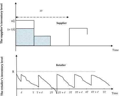
Figure 1. The supplier's replenishment system and the retailer's inventory policy

4-1 Decentralized Model

In the decentralized decision making structure, each SC member aims to optimize its own profit function. In the following, the SC member' profit function under decentralized model is calculated. In the decentralized model, the retailer acts as an SC leader and the supplier reacts as a follower. The retailer applies the periodic review inventory system (R, T) and decides on the review period (T) and order-up-to-level (R) along with the retail price (p_r) which have a considerable impact on the supplier's profitability. The retailer's order-up-to-level is calculated based on the expected demand within the protection interval demand (T + ℓ) as follow:

R = D(p_r)(T + ℓ) + kξ√T + ℓ (1) In addition, according to [Montgomery, Bazaraa, and Keswani, 1973] under the periodic

review inventory system, the expected holding cost (EHC) and the expected stock out cost (ESC) per year are calculated as Equations (2) and (3), respectively:

EHC = h_r[R − Dℓ −DT

2 + θE(X − R)+] (2)

ESC =π + θ(Pr− w)

T E(X − R)+

(3)

Consequently, the expected annual profit function of the retailer, π_r(T, R, p_r) under the periodic review inventory policy and partially lost sale can be formulated as:

(n-1)Q̅

nQ̅

2T + ℓ T

R

The r

etai

ler

's

inv

ento

ry

lev

el

Time Retailer

ℓ

The sup

pli

er'

s

inv

ento

ry

level

Time Supplier

3T

(9)

π_r(T, R, p_r)

= (p_r− w)D(p_r) −Ar T − h_r[R − D(p_r)ℓ −D(p₂r)T

+ θE(X − R)+_]

−π + θ(pr− w)

T E(X − R)+

(4)

The expected shortage quantity E(X − R)+ at the end of the cycle can be calculated as [Ouyang and Chuang, 2000]:

E(X − R)+_{= ∫ (X − R)}∞ R

f_xdx

= 𝜉√T + ℓψ(k) > 0

(5)

where, ψ(k) = φ(k) − k[1 − Φ(k)] and φ(k) and Φ(k) denote the standard normal and cumulative distribution functions, respectively. In the rest of this paper, for the sake of simplicity, the safety factor k will be used as a decision variable instead of the order-up-to-level R and hence π_r(T, R, p_r) can be converted to:

π_r(T, k, pr) = (pr− w)D(pr) − A_r

T − h_r[D(pr)T

2 + k𝜉√T + ℓ

+ θ𝜉√T + ℓψ(k)]

−1 T(π + θ(p_r

− w))𝜉√T + ℓψ(k)

(6)

in which, the first term denotes the retailer’s expected annual revenue. The second and third terms denote the expected annual ordering cost and annual holding cost, respectively. The last term denotes expected annual lost sales penalty and opportunity costs. According to Eq. (6), the retailer decides on T, k, and p_r to maximize its own profit function.

Proposition 1. The retailer profit function is strictly concave with respect to T, k, and 𝑝𝑟 under wide range of reasonable parameters.

Proof. See ‘‘Appendix 1’’.

By setting the ∂πr_∂T = 0,∂πr_∂k = 0,∂πr_∂pr = 0, the

optimal values of T, k, and pr can be obtained through Equations (7), (8), and (9), respectively.

A_r T2

=hrD(pr)

2 +

hrξ(k + θψ(k)) 2√T + ℓ

−(π + θ(pr− w))ξψ(k)√T + ℓ T2

+(π + θ(pr− w))ξψ(k) 2T√T + ℓ

(7)

1 − Φ(k)

= hr

h_rθ +1_{T (π + θ(p}_r− w))

(8)

pr= 𝒶 2Ɓ+

w 2 +

h_rT 4

−θξ√T + ℓψ(k) 2ƁT

(9)

Three equations (7), (8), and (9) are circularly dependent on each other. Thus, an algorithm as locally optimal algorithm is proposed to find the optimal solution of (T, k, pr) as follows:

Locally Optimal Solution Algorithm

Step 1: Input the values of all parameters;

Step 2: Set T be equal minimum feasible value;

Step 3: Set p_r= w;

Step 4: Calculate k using Eq. (8);

(10)

Step 6: Use a numerical search technique to obtain T which satisfies Eq. (7);

Step 7: Repeat third, fourth, fifth, and sixth steps to converge;

Step 8: The obtained T, k, and pr are optimum;

The optimal values of the retailer's decision variables are obtained from the above developed algorithm.

On the other side, the supplier applies a lot-for-lot replenishment system to replenish its inventory. The replenishment multiplier is assumed to be under the control of the supplier. The supplier receives the orders from the retailer in stable epochs, based on the retailer’s review periods. According to [Rosenblatt and Lee, 1985], the order multiplier n for the supplier must be a positive integer to optimize the supplier’s replenishment system. The supplier faces the ordering cost and holding cost. Hence, the expected annual profit function of the supplier, πs(n) can be formulated as follows:

π_s(n)

= (w − e)(D(p_r) −θ

Tξ√T + ℓψ(k)) −As

nT

− h_s[(n − 1) ((D(pr)T) − θξ√T + ℓψ(k))

2 ]

(10)

Proposition 2. The supplier profit function is concave with respect to n.

Proof: To prove concavity, it is assumed that 𝑛 is temporarily a continuous variable. Thus, the second order derivative of πs(n) with respect to 𝑛, will be:

∂2_π

s(n)

∂n2 = − 2A_s Tn3< 0

(11)

The second order derivative of πs(n) has a negative value. Therefore, the supplier profit function is concave with respect to 𝑛.

By setting ∂π_∂ns= 0, we have:

n = √ 2As

h_sD(p_r)T2_{− θξT√T + ℓψ(k)}

(12) The calculated 𝑛 maximizes the supplier profit function. Since, n is an integer variable thus, either the smallest following integer or largest previous integer of 𝑛 whichever results in larger value of πs(n) will be optimum value of 𝑛 from the supplier's perspective.

4-2 Centralized Model

Under the centralized decision making, it is assumed that all SC decisions are optimized from the whole SC view point. The expected annual profit function of SC can be calculated as the sum of the retailer’s annual expected profit and the supplier's annual expected profit as follows:

π_SC(T, k, p_r, n) = π_r(T, k, p_r) + π_s(n) = (p_r− e)D(p_r)

−1 T[Ar+

A_s n ]

−ξ√T + ℓψ(k)

T [(π

+ θ(p_r− e)) −hs(n − 1)θT

2 ]

−D(pr)T

2 [hr+ hs(n − 1)] − h_r[kξ√T + ℓ

+ θξ√T + ℓψ(k)]

(13)

Proposition 3. The supply chain profit function is concave with respect 𝑘, 𝑝_𝑟, 𝑎𝑛𝑑 𝑛 for a given T under wide range of reasonable parameters.

Proof. See ‘‘Appendix 2’’.

(11)

In addition, the optimal value of k is obtained

by setting ∂πSC_∂k = 0 as follows: 1 − Φ(k)

= hr

h_r_{θ + 1T[(π + θ(p}_r− e)) −hs(n − 1)θT

2 ]

(15)

Similarly, by setting ∂πSC

∂𝑝r = 0, the optimal value of 𝑝r is achieved:

p_r= 𝒶 2Ɓ+

e 2−

θ𝜉√T + ℓψ(k) 2ƁT +T

4[hr + h_s(n − 1)]

(16)

And also, by setting ∂πSC

∂n = 0 and releasing the constraint that n is an integer, the optimal value of 𝑛 is determined equal to Eq. (12).

Since the values of T, k, p_r, and n are circularly depending on each other, then an algorithm as the globally optimal algorithm is established to find the optimal solution of (T, k, p_r, n) as follows:

Globally Optimal Solution Algorithm

Step 1: Input the values of all parameters;

Step 2: Set T be equal minimum feasible value;

Step 3: Start with j=1 and the initial trial value of nj= 1;

Step 4: Set pj= w;

Step 5: Calculate kj using Eq. (15);

Step 6: Use the result in step 5, and then specify n_j+1 by Eq. (12) and p_j+1 by Eq. (16)

Step 7: If the difference between nj and nj+1 is sufficiently small (i.e.|nj− nj+1| ≤ 0.0001) then go to step 8. Otherwise, set j = j + 1 and then calculate pj+1 by Eq. (16) and go back to step 5;

Step 8: Calculate SC profit function using Eq. (13) according to the latest obtained T, k, pj, and n_j;

Step 9: If T > {(π + θ(pr− e))/(hr− θhr+

hs(n−1)θ

2 )} then terminate the algorithm; otherwise, T=T+ε (where ε is the lowest possible value for T) and go to Step 3;

Step 10: A combination of T, k, pr, and nj with the greatest SC profit function is optimal;

Hence, by considering the developed algorithm, the optimal values of T, k, pr, and n can be achieved which maximize the SC profit function as Eq. (17)

πSC(Tc, kc, prc, nc) ≥ πSC(Td, kd, prd, nd) (17)

Although applying Tc, kc, prc, ncincreases the SC profit function, it could incur losses for the retailer. As previously mentioned, the locally optimal decisions, Td, kd, prd, nd maximize the retailer profit function toward the globally optimal decisions, Tc, kc, prc, nc. That is,

π_r(Td_{, k}d_{, p}

rd) ≥ πr(Tc, kc, prc) (18)

It is clear that there is no incentive for the retailer to shift its local decisions to global decisions. In the following, a lead time reduction mechanism as an incentive scheme is offered by the supplier to induce the retailer to change its local decisions toward global decisions.

1 T2(Ar+

As n ) = [(π

+ θ(p_r− e))ξσψ(k)] ( 1 2T√T + ℓ

−√T + ℓ T2 ) −

h_s(n − 1)θξψ(k) 4√T + ℓ

+D(pr)

2 [hr+ hs(n − 1)] + h_r[ kξ

2√T + ℓ+

θξψ(k) 2√T + ℓ]

(12)

4-3 Coordinated Model: Lead Time

Crashing

Although the SC profitability increases under the centralized decision making model, this joint decision making structure could reduce the retailer's profitability. Thus, in this section, a lead time crashing as an incentive mechanism is offered by the supplier to convince the retailer to participate in the joint decision making model. As the lead time gets longer, the retailer must enhance its order-up-to-level in order to keep customer service level which incurs more inventory cost for the retailer. Thus, the lead time greatly affects the retailer's profitability. In the proposed incentive mechanism, the supplier aims to reduce the transportation lead time by spending more cost to motive the retailer to change its local decisions into global decisions. We consider the supplier reduces the transportation lead time through either the slow mode or the fast transportation mode similar to the work of Heydari, Zaabi-Ahmadi, and Choi [Heydari, Zaabi-Ahmadi, and Choi, 2016]. Through lead time reduction scheme the retailer’s inventory cost will be compensated by the supplier if spending more cost does not impose losses at supplier’s site. In other words, the proposed transportation lead time reduction must be satisfying for both the retailer and the supplier to participate in the coordination plan. Under coordinated decision making model, the expected retailer's profit function can be formulated as:

π_r(T, k, p_r)

= (pr− w)D(pr) − A_r

T − hr[

D(p_r)T

2 + kξ√T + ℓnew

+ θξ√T + ℓnewψ(k)] −1 T(π + θ(p_r− w))ξ√T + ℓnewψ(k)

(19)

In which ℓnew is considered as decreased lead time. Using the coefficient (1 − LTR) to reduce the general lead time leads to ℓnew,

Indeed crashing lead time from ℓ to ℓnew can increase the retailer's profit. If LTR becomes close to one, it can be concluded that the supplier decreases more lead time in order to enhance the retailer's profitability. On the other hand, if the LTR takes the value near zero, it implies that the supplier decreases lead time inconsiderably.

The retailer participates in the coordinated decision making model if its profitability increases towards the decentralized decision making model. Thus, the retailer's requirement for participation in the coordinated plan can be formulated as:

π_r(Tc_{, k}c_{, p}

rc, ℓnew ) ≥ πr(Td, kd, prd)

(21) By substituting Equations (6) and (19) into Eq. (21), the minimum value of the lead time reduction LTRmin can be determined as Eq. (22)

LTR_min= 1 − (((Y U)

2

− Tc_{) ×}1 ℓ)

(22)

Where,

Y = −Ar Tc+

A_r

Td− (prd− w)D(prd) + (p_rc_{− w)D(p}

rc)

− h_r(D(prc)Tc

2 )

+ h_r[D(prd)Td 2 + kd_ξ√Td_{+ ℓ}

+ θξ√Td_{+ ℓψ(k}d_{)] +}1 T(π + θ(p_rd

− w))ξ√Td_{+ ℓψ(k}d₎ (23)

(13)

U

= h_rkc_ξ+h

rθξψ(kc) +(π + θ(prc− w))

T ξ√Tc+ ℓψ(kc)

(24)

Using crashing lead time incurs more costs for the supplier. Thus the lead time crashing cost (LTCC) is incorporated into the supplier's profit function. As a result, the expected supplier's profit function can be calculated as follows:

In this paper (LTCC) function is calculated according to the work of Heydari, Zaabi-Ahmadi, and Choi [Heydari, Zaabi-Zaabi-Ahmadi, and Choi, 2016] which the lead time crashing cost is a function of transportation mode as well as lead time crashing. In addition, to create a realistic model, lead time crashing is considered thorough two ways as follows:

 Limited crashing without improving the transportation mode in which the cost of reduction linearly enhances and limits to the type of transportation mode.

 Additional decrease by altering the transportation mode which causes a fixed cost to the supplier.

Therefore, the lead time crashing cost function (LTCC) per cycle time can be formulated as Eq. (26)

In which M should be less than one and also the lead time reduction (LTR) should be in the interval (0, M). According to (LTTC) function, two transportation modes are considered: slow transportation mode and fast transportation mode where only F % reduction is conceivable without changing the transportation mode. While the lead time reduction (LTR) is in the interval [0, F], then the slow transportation mode (e.g. train) is proper. Moreover, if the lead time reduction (LTR) is in the interval [F, M] applying the fast transportation mode (e.g. truck) is appropriate.

The supplier offers the lead time crashing while its profitability increases towards the decentralized decision making model. Thus, the supplier's requirement for participation in the coordinated plan can be formulated as:

πs(Tc, kc, prc, nc, ℓnew ) ≥ πs(Td, kd, prd, nd) (27) Based on the supplier's profit function under the coordinated decision making model a closed-form equation for the maximum value of the lead time reduction LTR_max cannot be achieved. Thus, an algorithm is proposed to obtain LTR_max from the supplier's point of view.

Maximum Lead Time Reduction Algorithm

Step 1: Assign LTR=M;

Step 2: Calculate the supplier's profit function under the coordinated structure using Eq. (25);

Step 3: Check the supplier's participation constraint in Eq. (27);

Step 4: If the participation constraint (27) is not satisfied, then LTR=LTR-ε, (where ε is the small positive value), and go to Step 2; otherwise, the calculated value for LTR is LTR_max;

πs

= (w − e) (D(p_r) −θ_Tξ√T + ℓψ(k))

−As nT

− h_s[(n − 1) (D(pr)T − θξ√T + ℓψ(k))

2 ]

−LTCC T

(25) LTCC

= {_CR CRSL× LTR 0 < LTR ≤ F F× (LTR − F) + C + F × CRSL F < LTR ≤ M

(14)

Accordingly, all values of LTR in the interval [LTRmin, LTRmax] is capable of achieving channel coordination. At the lower bound, LTRmin, all the coordination profits will be obtained by the supplier. While at LTRmax, all the coordination profits will be gained by the retailer. The bargaining power of the retailer is considered ω against the supplier, hence the bargaining power of the supplier will be (1− ω). A linear profit sharing mechanism according to the members’ bargaining power is applied to find a proper LTR. Thus, based on the profit sharing strategy, LTR is achieved as Eq. (28)

LTR =

ω ×

LTR

_min

+ (1 −

ω

)

× LTR

max

(28)

5. Numerical Results

In order to demonstrate the performance and applicability of the developed models, test problems as well as a real case are prepared as follows. To solve the proposed models,

algorithms are run in MATLAB R2014b on the laptop with specification: core(TM) i3 CPU M370@ 2.40GHz and RAM 4.00 GB.

5-1 Numerical Experiments

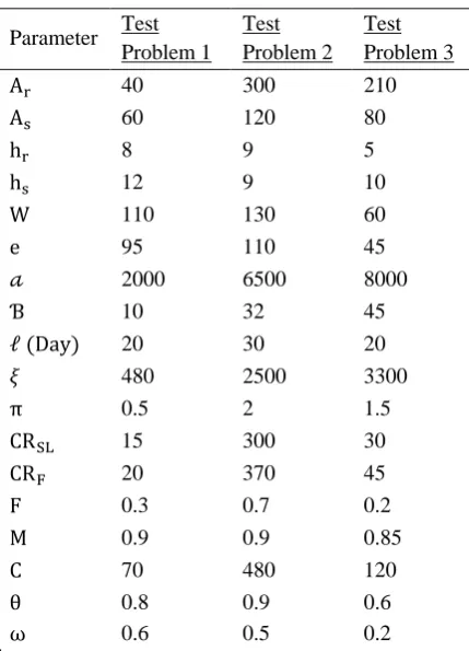
Data for the three test problems are shown in Table 2.

Table 2. Investigated test problems

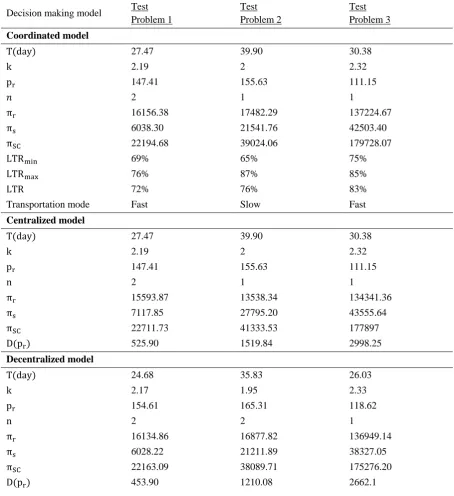
The results of running the developed models are indicated in Table 3. CPU time for solving three test problems are 37.461 s, 34.679 s, and 41.264 s, respectively. According to Table 3, in all test problems under the centralized decision making the SC profitability improves compared to the decentralized decision making. Indeed, the joint decision making can increase the market demand by reducing the retail price towards the decentralized setting as shown in Table 3. Thus, due to decreasing the retail price the retailer's profit decreases whereas the supplier benefits from joint decision making. In addition, lead time crashing as a coordination strategy is capable of ensuring the participation of two SC members in the joint decision making as well as improving the profitability of both SC members and SC profitability. According to test problems 1 and 2, although the lead time reduction scheme cannot increase the SC profitability compared to the centralized decision making, its cost is less than the achieved profit of the coordination plan on T, k, p_r, n. Lead time reduction mechanism is appealing for the retailer to accept the coordinated plan. Under test problem 3 applying lead time crashing as an incentive mechanism is able to achieve channel coordination as well as making more SC profitability in comparison with the centralized decision making. In other words, the supplier needs to spend lower cost than the achieved profit of the retailer.

A set of sensitivity analysis on the essential parameters is provided to demonstrate the applicability of the established models. According to the test problem 3, a set of

Parameter Test

Problem 1 Test Problem 2

Test Problem 3

Ar 40 300 210

As 60 120 80

hr 8 9 5

hs 12 9 10

W 110 130 60

e 95 110 45

𝒶 2000 6500 8000

Ɓ 10 32 45

ℓ (Day) 20 30 20

𝜉 480 2500 3300

π 0.5 2 1.5

CRSL 15 300 30

CRF 20 370 45

F 0.3 0.7 0.2

M 0.9 0.9 0.85

C 70 480 120

θ 0.8 0.9 0.6

(15)

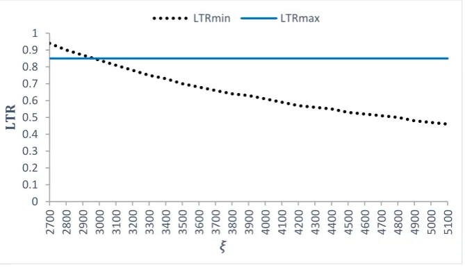
sensitivity analysis is conducted to investigate the effect of demand uncertainty, 𝜉 on the proposed models. Figure 2 illustrates the changes of the lead time reduction (LTR) as

demand uncertainty changes. As can be seen, by increasing the demand uncertainty the interval between LTRmin and LTRmax becomes larger.

Table 3. Results of running the three decision making models under three investigated test problems

A set of sensitivity analysis on the essential parameters is provided to demonstrate the applicability of the established models. According

to the test problem 3, a set of sensitivity analysis is conducted to investigate the effect of demand uncertainty, 𝜉 on the proposed models. Figure 2

Decision making model Test

Problem 1

Test Problem 2

Test Problem 3 Coordinated model

T(day) 27.47 39.90 30.38

k 2.19 2 2.32

pr 147.41 155.63 111.15

𝑛 2 1 1

πr 16156.38 17482.29 137224.67

πs 6038.30 21541.76 42503.40

πSC 22194.68 39024.06 179728.07

LTRmin 69% 65% 75%

LTRmax 76% 87% 85%

LTR 72% 76% 83%

Transportation mode Fast Slow Fast

Centralized model

T(day) 27.47 39.90 30.38

k 2.19 2 2.32

pr 147.41 155.63 111.15

n 2 1 1

πr 15593.87 13538.34 134341.36

πs 7117.85 27795.20 43555.64

πSC 22711.73 41333.53 177897

D(pr) 525.90 1519.84 2998.25

Decentralized model

T(day) 24.68 35.83 26.03

k 2.17 1.95 2.33

pr 154.61 165.31 118.62

n 2 2 1

πr 16134.86 16877.82 136949.14

πs 6028.22 21211.89 38327.05

πSC 22163.09 38089.71 175276.20

(16)

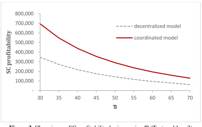
illustrates the changes of the lead time reduction (LTR) as demand uncertainty changes. As can be seen, by increasing the demand uncertainty the interval between LTRmin and LTRmax becomes larger. In addition, there exist a junction point between LTRmin and LTRmax lower that applying lead time crashing scheme incurs more cost for the supplier compared to the achieved profit of joint decision making. Thus, at lower values of this junction point the coordination plan will not be reached since LTR_min is greater than LTR_max. Accordingly, the proposed model is applicable if LTRmax is bigger than LTRmin. Hence, it can be concluded that the developed coordination model could be of high applicability when the supply chain faces a stochastic demand. Furthermore, to demonstrate the effect of price-elasticity coefficient of demand, Ɓ on the developed models a sensitivity analysis is provided with respect to test problem 3. Figure 3 depicts the changes in the whole SC profitability as Ɓ changes. As shown in Figure 3, although by

increasing Ɓ, the SC profitability diminishes in the decentralized and coordinated models but the coordination model can remove the negative effects of increasing Ɓ on the SC profitability towards the decentralized decision making. Thus, the proposed coordination model is of high benefit for the supply chain when it faces a price sensitive demand. In addition, a set of sensitivity analysis on the crucial parameters, CRSL, CRF, C, and F is carried out to demonstrate the applicability of the developed models. Parameters for these analyses are taken from the test problem 1 and the sensitivity results of the mentioned parameters are illustrated in Figure 4a to Figure 4.d, respectively. According to Figure 4a, as CR_SL increases, LTRmax closes LTRmin. According to this figure, LTRmax decreases by increasing CR_SL. Although in a high value of CR_SL, LTRmax is smaller than LTRmin which implies that in the greater amount of CRSL the channel coordination will not be achieved.

Figure 2. Values of LRTminand LTRmax by changing uncertainty (𝜉) (Test problem 3)

0 0.1 0.2 0.3 0.4 0.5 0.6 0.7 0.8 0.9 1

2700 2800 2900 3000 3100 3200 3300 3400 3500 3600 3700 3800 3900 4000 4100 4200 4300 4400 4500 4600 4700 4800 4900 5000 5100

LTR

𝜉

(17)

153 International Journal of Transportation Engineering, Vol. 5/ No. 2/ Autumn 2017 Figure 3. Changing on SC profitability by increasing Ɓ(Test problem 3)

Thus, the coordination model is applicable and economical for the supply chain when the supplier by crashing lead time incurs small values of CR_SL.

Further, Figure 4b, indicates the changes of LTR_min and LTR_max by changing CR_F. As illustrated in Figure 4.b as CR_F increases LTR_max decreases. Moreover, in the high value of CRF the proposed coordination model cannot be reached due to the interval of [LTRmin, LTRmax] is empty. Thus, the proposed coordination model is applicable and economical for the supply chain when the supplier faces small values of CRF under lead time reduction.

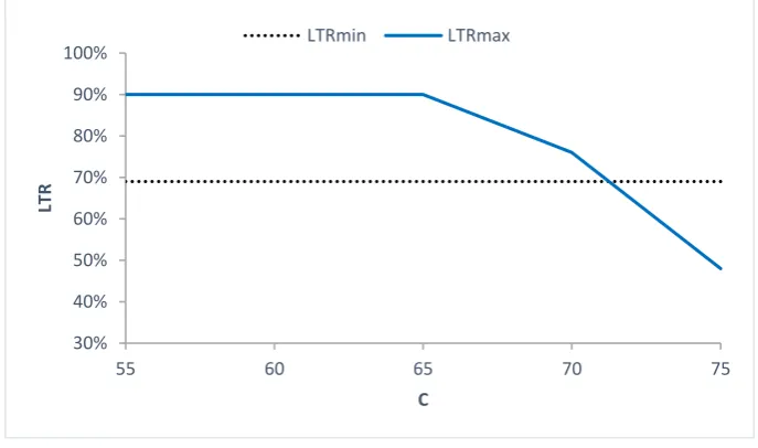
Figure 4c, shows the changes of LTRmin and LTR_max by changing C, fixed cost for switching from slow transportation mode to fast mode. As illustrated in Figure 4c, in the smaller value of C than 70, the amount of LTR is more than F% (F=0.3 according to test problem 1), indicating the supplier intends to switch the transportation

mode. Although in the high value of C improving the transportation mode will not be economical for the supplier. Accordingly, the proposed coordination model is of great benefit for the supply chain in which the supplier faces small values of switching the transportation mode.

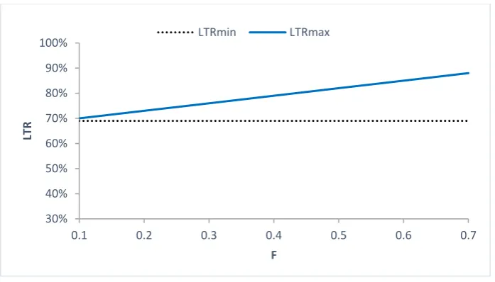
Eventually, the changes of LTR_min and LTR_max versus changing F is shown in Figure 4d. According to Figure 4d, as F increases LTRmax increases too. In the value of F=10%, LTRmax is equal to F whereas in the high values of F, LTRmax will linearly increase. In other words, growing F implies that applying lead time crashing does not need improvement in the transportation mode which in turn makes lower cost for the supplier. As a result, the developed coordination model is of high applicability for the supply chain when it faces high value of F in which more lead time reduction is conceivable without enhancing the transportation mode.

100,000 200,000 300,000 400,000 500,000 600,000 700,000 800,000

30 35 40 45 50 55 60 65 70

SC

profitabi

lity

Ɓ

decentralized model

(18)

Figure 4a. Values of LRTminand LTRmax by increasing CRSL (Test problem 1)

Figure 4b. Values of LRTminand LTRmax by increasing CRF (Test problem 1)

Figure 4c. Values of LRTminand LTRmax by increasing C (Test problem 1) 30%

40% 50% 60% 70% 80% 90% 100%

5 10 15 20 25

LTR

CRsl

LTRmin LTRmax

30% 40% 50% 60% 70% 80% 90% 100%

5 10 15 20 30

LTR

CRf

LTRmin LTRmax

30% 40% 50% 60% 70% 80% 90% 100%

55 60 65 70 75

LTR

C

(19)

155 International Journal of Transportation Engineering, Vol. 5/ No. 2/ Autumn 2017 Figure 4d. Values of LRTminand LTRmax by increasing F (Test problem 1)

5-2 Case Study

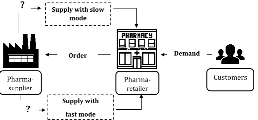
This section conducts a real problem in order to better demonstrate the performance of the proposed incentive mechanism. The problem includes a pharma-retailer (pharmacy) which supplies its medicines from a pharma-supplier (pharmaceutical company). Indeed, the mentioned real problem associated with a pharmaceutical supply chain (PSC) as illustrated in Figure 5. For a specific medicine (Dexamethasone ampoule), the pharma-retailer faces a stochastic price dependent demand following a normal distribution. Dexamethasone is the most effective and safe medicines needed in a health system. It is applied in the treatment of many conditions such as a number of skin diseases, asthma, and severe allergies. Due to the long transportation lead time, the pharma-retailer needs to stock more inventory which in turn imposes high inventory cost. Hence, the lead time affects the PSC members' profitability and the PSC decisions as well.

 Pharma-retailer objective: The pharma-retailer aims to maximize its profit function to obtain its optimal decision variables: review period (T), order-up-to-level), and retail price. Although, these decisions

impact the pharma-supplier's decisions as well as PSC profitability.

 Pharma-supplier objective: The pharma-supplier seeks to maximize its profit function in order to find the optimal decision variable: number of replenishments (n).

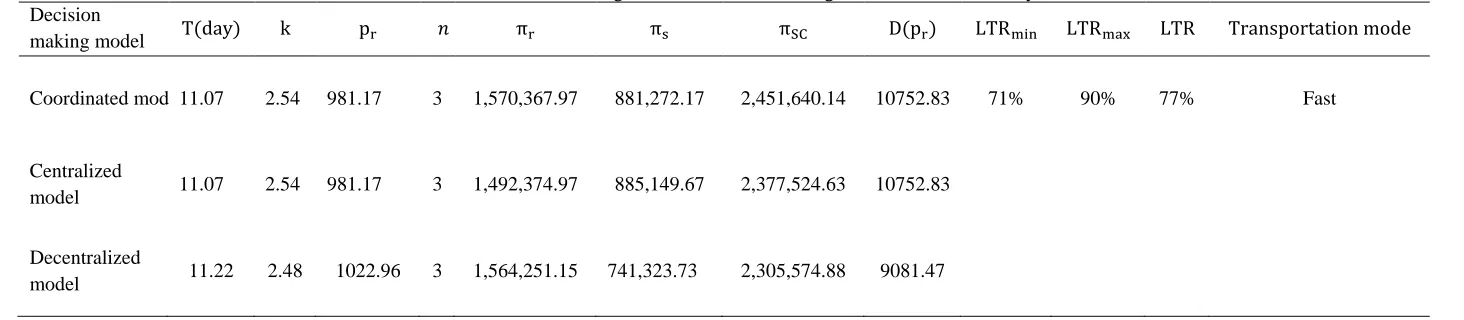
According to the described real problem we aim to propose the best optimal solution for both pharma members as well as entire PSC. To this end, we investigate the PSC model, under three decision making models, i.e., decentralized, centralized, and coordinated models. The parameters of the real problem are shown in Table 4. In addition, the obtained results of the running three decision making structures, i.e. decentralized, centralized, and coordinated models are illustrated in Table 5.

Under the decentralized decision making model in which each pharma member makes decisions individually regardless of the other PSC members. Since these decisions are made individually are not optimal from the whole PSC perspective.

Under centralized decision making structure, all PCS decisions are made from the PSC view point. Although, this joint decision improves PSC profitability as well as pharma-supplier. The pharma-retailer incurs losses. As a result, the 30%

40% 50% 60% 70% 80% 90% 100%

0.1 0.2 0.3 0.4 0.5 0.6 0.7

LTR

F

(20)

pharma-retailer does not accept the joint decision making model. Thus, an incentive mechanism needs to convince the pharma-retailer to change the local decisions (decentralized decision making model) toward the global decisions (centralized decision making model). To this end, we suggest an incentive mechanism through lead time crashing to coordinate the pricing and replenishment decisions along with the PSC profitability as well as the profitability of both PSC members ensured.

According to the developed incentive mechanism, the pharma-supplier seeks to reduce the transportation lead time by spending more cost under the transportation mode selection. In other words, the pharma-supplier applies two transportation modes: slow transportation mode and fast transportation mode which uses a slow mode for a certain lead time threshold and for the greater lead time reduction exerts a fast mode transportation.

Implementing the suggested lead time reduction scheme under the mentioned real problem can improve the PSC profitability as well as the profitability of both PSC members. Moreover, the proposed coordination plan is able to achieve channel coordination for the PSC. Hence, both PSC members are motivated by the suggested incentive scheme to make decisions jointly. Moreover, the coordination parameters, LTR_min and LTRmax are derived from the retailer’ view point and pharma-supplier's perspective as shown in Table 5. According to our proposed model, the obtained value of LTR demonstrates that the pharma-supplier should choose the fast transportation mode to reduce the transportation lead time. Moreover, the suggested lead time crashing spends lower cost for the pharma-supplier towards the achieved benefit for the pharma-retailer and results in achieving channel coordination

Figure 5. The two echelon pharmaceutical supply chain model Supply with slow

mode

Supply with

fast mode

Order Demand

?

Pharma

-supplier

Pharma

-retailer

(21)

157 International Journal of Transportation Engineering, Vol. 5/ No. 2/ Autumn 2017 Table 4. Parameters of case study

parameters Ar As hr hs W e 𝒶 Ɓ ℓ (Day) 𝜉 π CRSL CRF F M C θ ω

2000 800 50 20 800 715 50000 40 10 11500 8 45 90 0.4 0.9 150 1 0.7

Table 5. Results of running the three decision making models under case study Decision

making model T(day) k pr 𝑛 πr πs πSC D(pr) LTRmin LTRmax LTR Transportation mode

Coordinated model 11.07 2.54 981.17 3 1,570,367.97 881,272.17 2,451,640.14 10752.83 71% 90% 77% Fast

Centralized

model 11.07 2.54 981.17 3 1,492,374.97 885,149.67 2,377,524.63 10752.83

Decentralized

(22)

6. Conclusion

In this paper, a transportation lead time reduction scheme was developed to coordinate a supplier-retailer chain. In our investigated SC, the supplier-retailer faced the periodic review inventory policy (R, T) in which both the review period (T) and order-up-to-level (R) were retailer's decision variables along with the retail price. In addition, the customers' demand was considered to be stochastic and price dependent. Whereas the supplier used a lot-for-lot replenishment system and decided on the replenishment multiplier. The lead time consisted of one component: transportation time which was under the control of the supplier. Our proposed SC was modeled under three different decision making structures: (1) decentralized, (2) centralized, and (3) coordinated structures. We suggested a lead time reduction strategy as an incentive scheme to guarantee the participation of two SC members in the joint decision making. Through the proposed incentive mechanism, the supplier aimed to reduce the transportation lead time by spending more cost and also enhancing the transportation mode to entice the retailer to change the locally decision making toward the joint decision making. Moreover, in the proposed incentive scheme, two transportation modes (one slow and one fast) were supposed. In our investigation, the supplier applied a certain transportation mode for a specific lead time reduction and for more crashing lead time improved the transportation mode by switching to fast mode. To create a realistic model, in our proposed incentive scheme, the lead time crashing cost was considered. Furthermore, a set of numerical examples along with a real case were conducted to demonstrate the performance and applicability of the developed models. The results demonstrated that the developed incentive scheme can ensure more SC profitability as well as SC members. Moreover, the results indicated the applicability of the suggested coordination plan when the SC faced high demand

uncertainties. The obtained results revealed that the pricing decision was as important as the replenishment decisions in the supply chain due to the significant impacts on the SC profitability. In addition, the proposed coordination model could share the obtained profits between two SC members fairly.

This investigation can be extended by considering a game-theoretic analyses of lead time crashing. Moreover, this paper can be expanded by considering other lead time elements such as set up lead time, production lead time, loading or unloading lead time and so forth.

7. References

Ai, X., Chen, J., Zhao, H. and Tang, X. (2012) “Competition among supply chains: implications of full returns policy” International Journal of Production Economics, Vol. 139, No. 1, pp. 257-265.

Arani, Vafa, H., Rabbani, M. and Rafiei, H. (2016) “A revenue-sharing option contract toward coordination of supply chains”, International Journal of Production Economics, Vol. 178, pp. 42-56.

Arkan, A. and Hejazi, S. R. (2012) “Coordinating orders in a two echelon supply chain with controllable lead time and ordering cost using the credit period”, Comput Ind Eng, Vol. 62, pp. 56–69.

Boyacı, T. and Gallego, G. (2002) “Coordinating pricing and inventory replenishment policies for one wholesaler and one or more geographically dispersed retailers”, International Journal of Production Economics, Vol. 77, No. 2, pp.95-111.

Chaharsooghi, S. K. and Heydari, J. (2010a) “Optimum coverage of uncertainties in a supply chain with an order size constraint”, The International Journal of Advanced Manufacturing Technology, Vol. 47, No. 1-4, pp. 283-293.

(23)

Chaharsooghi, S.K., Heydari, J. and Kamalabadi, I.N. (2011) “Simultaneous coordination of order quantity and reorder point in a two-stage supply chain”, Computers & Operations Research, Vol. 38, No. 12, pp. 1667-1677.

Chen, T.H. and Chang, H.M. (2010) “Optimal ordering and pricing policies for deteriorating items in one-vendor multi-retailer supply chain”, The International Journal of Advanced Manufacturing Technology, Vol. 49, No. 1-4, pp. 341-355.

Cohen, M. A. (1977) “Joint pricing and ordering policy for exponentially decaying inventory with known demand”, Naval Research Logistics Quarterly, Vol. 24, No. 2, pp.257-268.

Du, R., Banerjee, A. and Kim, S.L. (2013) “Coordination of two-echelon supply chains using wholesale price discount and credit option”, International Journal of Production Economics, Vol. 143, No. 2, pp.327-334.

Dumrongsiri, A., Fan, M., Jain, A. and Moinzadeh, K. (2008) “A supply chain model with direct and retail channels”, European Journal of Operational Research, Vol. 187, pp. 691-718.

Emmons, H. and Gilbert, S. M. (1998). “Note. The role of returns policies in pricing and inventory decisions for catalogue goods”, Management Science, Vol. 44, pp. 276-283.

Giri, B.C. and Maiti, T. (2013). “Supply chain model with price-and trade credit-sensitive demand under two-level permissible delay in payments”, International Journal of Systems Science, Vol. 44, No. 5, pp. 937-948.

Heydari, J. (2014a) “Coordinating supplier׳ s reorder point: A coordination mechanism for supply chains with long supplier lead time”, Computers & Operations Research, Vol. 48, pp. 89-101.

Heydari, J. (2014b) “Lead time variation control using reliable shipment equipment: An incentive scheme for supply chain coordination”, Transportation Research Part E: Logistics and Transportation Review, Vol. 63, pp. 44-58.

Heydari, J. (2015) “Coordinating replenishment decisions in a two-stage supply chain by considering truckload limitation based on delay in payments”, International Journal of Systems Science, Vol. 46, No. 10, pp. 1897-1908.

Heydari, J. and Norouzinasab, Y. (2015) “A two-level discount model for coordinating a decentralized supply chain considering stochastic price-sensitive demand”, Journal of Industrial Engineering International, Vol. 11, No. 4, pp. 531-542.

Heydari, J. and Norouzinasab, Y. (2016) “Coordination of pricing, ordering, and lead time decisions in a manufacturing supply chain”, Journal of Industrial and Systems Engineering, Vol. 9, pp. 1-16.

Heydari, J., Zaabi-Ahmadi, P. and Choi, T.M. (2016) “Coordinating supply chains with stochastic demand by crashing lead times”, Computers & Operations Research.

Hojati, S., Seyedhosseini, S.M., Hosseini-Motlagh, S.M. and Nematollahi, M.R. (2017) “Coordination and profit sharing in a two-level supply chain under periodic review inventory policy with delay in payments contract”, Journal of Industrial and Systems Engineering, Vol. 10

Johari, M., Hosseini-Motlagh, S.M. and Nematollahi, M.R. (2017) “Simultaneous coordination of review period and order-up-to-level in a manufacturer-retailer chain”, Journal of Industrial and Systems Engineering, Vol. 10, special issue on production and inventory, pp 1-17.

Leng, M. and Parlar, M. (2009) “Lead-time reduction in a two-level supply chain: Non-cooperative equilibria vs. coordination with a profit-sharing contract”, International Journal of Production Economics, Vol. 118, No. 2, pp. 521-544.

Li, Y., Xu, X., Zhao, X., Yeung J. H. Y. and Ye, F. (2012) “Supply chain coordination with controllable lead time and asymmetric information”, Eur J Oper Res, Vol. 217, pp. 108–19.

(24)

Mokhlesian, M., Zogordi, S.H., Nakhai Kamal Abadi, I. and Albadvi, A. (2015) “Pricing decisions in a two-echelon decentralized supply chain using bi-level programming approach”, Journal of Industrial and Systems Engineering, Vol. 8, No. 1, pp. 106-124.

Nematollahi, M., Hosseini-Motlagh, S.M. and Heydari, J. (2017a) “Coordination of social responsibility and order quantity in a two-echelon supply chain: A collaborative decision-making perspective”, International Journal of Production Economics, Vol. 184, pp. 107-121.

Nematollahi, M., Hosseini-Motlagh, S.M. and Heydari, J. (2017b) “Economic and social collaborative decision-making on visit interval and service level in a two-echelon pharmaceutical supply chain”, Journal of Cleaner Production, Vol. 142, Part 4, pp. 3956-3969.

Ouyang, L. Y. and Chuang, B. R. (2000) “A periodic review inventory model involving variable lead time with a service level constraint”, International Journal of Systems Science, Vol. 31, No. 10, pp. 1209-1215.

Panda, S. (2014) “Coordination of a socially responsible supply chain using revenue sharing contract”, Transp. Res. Part E, Vol. 67, pp. 92–104.

Rosenblatt, M. J. and Lee, H. L. (1985), “Improving profitability with quantity discounts under fixed demand”, IIE Transactions, Vol. 17, pp. 388–395.

Rushton, A., Croucher, P. and Baker, P. (2010) “The handbook of logistics and distribution management: Understanding the supply chain”, UK: Kogan Page Publishers.

Sajadieh, M.S. and Akbari Jokar, M. R. (2009) “Optimizing shipment, ordering and pricing policies in a two-stage supply chain with price-sensitive demand”, Transportation Research Part E: Logistics and Transportation Review, Vol. 45, No. 4, pp. 564-571.

Seifbarghy, M., Nouhi, K. and Mahmoudi, A. (2015) “Contract design in a supply chain considering price and quality dependent demand with customer segmentation”, International Journal of Production Economics, Vol. 167, pp. 108-118.

Sinha, S. and Sarmah, S. P. (2010) “Coordination and price competition in a duopoly common retailer supply chain”, Computers & Industrial Engineering, Vol. 59, No. 2, pp. 280-295.

Yang, P.-Ch. (2004) “Pricing strategy for deteriorating items using quantity discount when demand is price sensitive”, European Journal of Operational Research, Vol. 157, No. 2, pp. 389-397.

Appendix 1

(25)

r

r r _r

2_π 2_π 2_π

r r r

2 k T p

2_π 2_π 2_π

r r r

πr _{k T} ₂ _{k p}

k

2_π 2_π 2_π

r r r

p T T T

(

2

p _p

)

k H

 

 

 

  

    

  

  _  

  

    _



in which,

∂2_π

r(T, k, Pr)

∂T2 =

−2A_r T3

+ [ 1

T2_{√T + ℓ}−

2√T + ℓ

T3 +

1

4T(T + ℓ)32

] ((π + θ(P_r− w))ℓψ(k))

+hrℓ(k + θψ(k)) 4(T + ℓ)32

(1a)

According to Eq. (7) in section 4, this implies that,

if let,

and

then,

On the other hand, A_r

2T2_{(T + ℓ)}+

(π + θ(p_r− w))𝜉ψ(k)√T + ℓ

2T2_{(T + ℓ)} −

(π + θ(p_r− w))𝜉ψ(k)

4T(T + ℓ)32

>hr𝜉(k + θψ(k)) 4(T + ℓ)

(2a)

E1 =2Ar T3 − [

1 T2_{√T + ℓ}−

2√T + ℓ

T3 +

1

4T(T + ℓ)32

] ((π + θ(P_r− w))𝜉ψ(k))

(3a)

E2 = Ar

2T2_{(T + ℓ)}+

(π + θ(P_r− w))𝜉ψ(k)√T + ℓ

2T2_{(T + ℓ)} −

(π + θ(P_r− w))𝜉ψ(k)

4T(T + ℓ)32

(4a)

E3 = E1 −hr𝜉(k + θψ(k)) 4(T + ℓ)32

(5a)

∂2_π

r(T, k, Pr)

∂T2 = −E3

(26)

from the above we have,

hence, the first principal minor (|H11|) is negative as follows:

The second principle minor (|H22|) is positive when:

The condition is tested numerically and observed that it would be satisfied for a wide range of reasonable parameters and considered test problem.

And the third principle minor (|H33|) is negative when:

These conditions are tested numerically and observed that it would be satisfied for a wide range of reasonable parameters and considered test problem as illustrated in Table A1. Then, by satisfying conditions (10a) and (11a) Hessian matrix of the retailer expected annual profit function is negative definite.

Table A1. Results of Hessian matrix of the retailer profit function under three test problems

Test problems Second principle minor (H22) Third principle minor (H33)

1 137001375 -2959021689

2 2938262630 -159967709035

3 2363524155 -244631317012

E2 >hr𝜉(k + θψ(k)) 4(T + ℓ)32

(7a)

E3 > E1 − E2 =Ar(3T + 4ℓ) 2T3_{(T + ℓ)} +

(π + θ(P_r− w))𝜉ψ(k)(4ℓ + T)

2T3_{√T + ℓ} > 0

(8a)

|H₁₁| =∂2πr(T, k, Pr) ∂T2 < 0