Automatic formulation of falling multiple flexible-link robotic manipulators using 3×3 rotational matrices

I S A V

Journal of Theoretical and Applied

Vibration and Acoustics

journal homepage: http://tava.isav.ir

Automatic formulation of falling multiple flexible-link robotic

manipulators using 3×3 rotational matrices

Ali Mohammad Shafei

*

Assistant Professor, Department of Mechanical Engineering, Shahid Bahonar University of Kerman, Kerman, Iran

A R T I C L E I N F O A B S T R A C T

Article history:

Received 15 January 2016

Received in revised form 28 October 2016

Accepted 4 November 2016

Available online 15 March 2017

In this paper, the effect of normal impact on the mathematical modeling of flexible multiple links is investigated. The response of such a system can be fully determined by two distinct solution procedures. Highly nonlinear differential equations are exploited to model the falling phase of the system prior to normal impact; and algebraic equations are used to model the normal collision of this open-chain robotic system. To avoid employing the Lagrangian

method which suffers from too many differentiations, the governing

equations of such complicated system are acquired via the Gibbs-Appell (G-A) methodology. The main contribution of the present work is the use of an automatic algorithm according to 3×3 rotational matrices to obtain the system’s motion equations more efficiently. Accordingly, all mathematical formulations are completed by the use of 3×3 matrices and 3×1 vectors only. The dynamic responses of this system are greatly reliant on the step sizes. Therefore, as well as solving the obtained differential equations by using several ODE solvers, a computer program according to the Runge-Kutta method was also developed. Finally, the computational counts of both algorithms i.e., 3×3 rotational matrices and 4×4 transformation matrices are compared to prove the efficiency of the former in deriving the motion equations.

©2017 Iranian Society of Acoustics and Vibration, All rights reserved. Keywords:

Recursive formulation

Gibbs-Appell

Impact phase

Flying phase

3×3 rotational matrices

* Corresponding author.

E-mail address: [email protected] (A. M. Shafei)

16

1. Introduction

When a mechanical system is subjected to applied impulses or the constraints on the system are abruptly varied, the velocity of the components in the system changes so rapidly that the duration of the process may be considered to be instantaneous. The mathematical modeling of ground collision in open chain robotic systems constructed of flexible links has diverse applications. For example, in the dynamic modeling of biped robotic systems, it is essential to know the dynamic responses of the system at the impact moments. In fact, the viscoelastic properties of human muscles that cover the bones justify the use of flexible links to model the bipedal robotic systems.

Unlike the classical problem of collision between two objects, a small amount of literature exists about the impact phenomenon in robotic systems. In an early study of this subject, Wittenburg [1] employed the Newton-Euler’s methodology to obtain the governing equations at impact moments. Chang and Peng [2] exploited the Kane’s formulation to investigate the impulsive motion in robotic systems by considering four various kinds of impulsive constraints. Mathematical modeling of frictional impacts in robotic manipulators have been studied by Hurmuzlu and Marghitu [3]. They developed three dynamical models for the coefficient of restitution according to the Newton’s model of restitution. Rodriguez and Bowling [4] presented multi-point models of impact in rigid body systems. In this work, the effect of friction was also considered. The dynamic behavior of robotic manipulators with flexible joints colliding with their confining walls has been studied by Mahmoodi et al. [5]. In their paper, an adaptive controller is suggested to accomplish trajectory tracking of this robotic system. Shafei and Shafei [6] studied the effects of impact in open-chain robotic systems with flexible links. To simulate the conditions under which a single flexible link strikes with multiple flat confining walls, they employed the Newton’s impact law. However, the chief objective of all the aforementioned studies has been to better the modeling of impact in robotic manipulators with finite numbers of rigid or flexible links; and robotic systems with many degrees of freedom have not been considered.

17 The two chief questions in multi-flexible-link robotic manipulators with impulsive constraints are: 1) How to construct a valid elasto-dynamic model with the acceptable computational counts, and 2) How to incorporate the algebraic equations of this multi-flexible-link robotic arm into the relevant differential equations. In most of mechanical systems, it is essential to model the system as precise as possible. When more bodies are employed in dynamic modeling a robotic system, the mathematical operations needed to obtain the motion equations grow rapidly. Therefore, it is crucial to exploit an automatic algorithm to derive the motion equations, as fast as possible. There are many formulations that are effective in deriving the governing equations of open-chain robotic systems [18-24]. A comprehensive literature survey of the different recursive algorithms for elastic robotic manipulators may be found in [25]. Nevertheless, the stress of this paper is on the Gibbs-Appell formulation which has been used the least among the other method. Recently, Korayem and Shafei effectively applied this methodology for systematic formulation of flexible robotic arms [26-28], mobile robotic manipulators [29-31] and manipulators with revolute-telescopic joints [32, 33]. However, in none of these works the effects of impact between a manipulator and the ground have been considered.

The governing motion equations of robotic arms consisting of the unilateral constraints have formerly been fully formulated. The finite and impulsive motions of robotic arms with impacts can be characterized by differential and algebraic equations, respectively. However, the implementation of these differential-algebraic equations is restricted by significant computational load especially when the number of shape functions used to model the elastic properties of the flexible links increases. Consequently, researchers have concentrated to better the algorithms in order to simulate more complicated robotic systems with impact phenomenon. Förg et al. [34] suggested an algorithm for robotic systems with several constraints to treat many impacts. An O

 

n recursive algorithm according to the Projection Equation was offered by Gattringer et al. [35]. By using the Dirac delta functions, Tlalolini et al. [36] modeled the external forces originating from the collision of a thirteen-link humanoid robotic system with the ground. They exerted a Newton-Euler formulation in recursive form to extend an optimization algorithm for specifying the optimal cyclic gaits of the robot. Also, in the work of Shafei and Shafei [37], the mathematical model of multi-flexible-links subjected to impact was extracted in a symbolic format by employing the Gibbs-Appell formulation and 4×4 transformation matrices. However, despite using compact formulas in their work, the developed algorithm had a high computational complexity. Anyway, in all of the above-mentioned studies, the results of the impact model that should be exploited to characterize the generalized velocities of the system after impact moment, have not been formulated by an efficient algorithm with the least number of mathematical operations.

18

2. Kinematics of a falling down multi-flexible link

2.1. System specifications

This section presents the kinematics of a planar robotic arm which constructed by flexible links and floated through the space. Link (i1) and Link (i ) of this robotic system are depicted in Fig. 1. Two moving frames (x_i,1x_i,2x_i,3,xˆ_i,1xˆ_i,2xˆ_i,3) are assigned to each elastic link according to the forthcoming rules. x_i,1x_i,2x_i,3 is the moving frame for the ith link that its origin is located at the start of this body; the x_i,1 axis is along the link when it is undeformed and the x_i,3 axis is aligned the joint axis. On the other hand, the origin of xˆ_i,1xˆ_i,2xˆ_i,3 moving frame is situated to the end of this link and its orientation is precisely the same as the xi,1xi,2xi,3 moving frame, when this link has no deformation. Finally, refX₁refX₂refX₃ is the coordinate system which is devoted to the ground, as the global reference frame. In this paper, it is supposed that the manipulator has a moving base and consequently can easily move. So, the position and velocity of O1 with respect to the inertia reference frame are respectively denoted by X_j and Xj, where j 1,2. It is

emphasized, the elastic attributes of the flexible links (i.e., modulus of elasticity E_i and modulus of rigidity G_i), mass per unit length (_i) and mass moment of inertia per unit length (J_i) are assumed to be isotopic along the links. Here, the elastic property of each link is modeled with the same number of shape functions (m). So, the degree of freedom (D.O.F) for the system is:

2

  n nm

DOF where n D.O.F are related to the joint angles (q_j), nm D.O.F of the system are related to the small deflections of the links (_ij)and the remaining two D.O.F are associated with the position of the start point (O₁) with respect to the global coordinate system (X_j).

2.2. Kinematic equations

In Fig. 1, a differential element, Q, is demonstrated. The location of this differential element with respect to the x_i,1x_i,2x_i,3 moving frame can be represented as,

   

   

     

Elastic m

j ij ij Rigid

i i i Q/O

i _{η δ t η}

i  x,1



1 r r

(1)

19

Fig. 1. A falling down multi-flexible links

   

t η δ _ij m

j ij i

i_θ



_θ





1 (2)

i

O

1 

i

O 1



i

O

Q

 

 _yi

 d

Q zi

 



 d

Q

i

O Q i

/ r

g

i

q_

1



i

q_

1



i

q ij

 j

i1



 

 zi

 

 _yi

1 O to

1 

n

O to

1 , 1 

i

x 2

, 1 

i

x

1 , i x 2 , i

x

1 , 1 ˆ_i

x 2

, 1 ˆ_i

x

1 , ˆ_i

x 2 , ˆ_i

x

1



i Link

i Link

centerline to

Tangent

centerline with

Parallel 1

, i

x with Parallel

2 , i

x with Parallel

3 , i

x with Parallel

1 , 1 ˆ

x

1 , 1 x

2 , 2 x

3 , 2 3 , 1 ,

ˆ x

x

1

q

2

q j

1



1 O

2 O 2 , 1 ˆ x

1

Link

2

Link 2

, 1 x

3 , 1 x

1 X

ref 2 X

ref

1 X

2 X

1 X 2

X

20 where _ij



θ_xij θ_{x ij} θ_xij



T

3 2 1



θ is the eigen function vector which includes rotational shape

functions (θ_xij

1 , θx2ij and θx3ij) in principle axes (Oixi,1, Oixi,2 and Oixi,3).

As the approach proposed in this paper is according to the G-A methodology, the absolute acceleration of Q is needed. This term can be expressed as,



_i



i i

i

i Q/O

i i i i i Q/O i i i Q/O i i i Q/O i O i Q

i_{r r r  ωr ωr ω  ωr}

  



 2 ₍₃₎

where O_i i_r

 is the acceleration of the ith joint and iω_i is the angular velocity of the ith link. Also,

i

Q/O i_r

 and Q/O_i i_r

 can be obtained by once and twice differentiating of Eq. (1), respectively. In following section, Eq. (3) will be employed to establish the Gibbs function (acceleration energy) of the system.

3. Dynamics of a falling down multi-flexible link

In this section, two dynamical models, namely, flying phase and impact phase are developed to study the dynamic behavior of multi-flexible-link robotic systems. The finite motion of the above-mentioned robotic system during the flying phase will be obtained by differential equations, while the impulsive motion due to the collision of this mechanical system with the ground will be formulated by algebraic equations. In below, the details of these two phases are described.

3.1. Dynamics of the system in the flying phase

In the flying phase, the manipulator is suspended through the space and has no contact with the ground [38]. In this paper, differential equations for the flying phase are attained by the G-A formulation, in which the acceleration energy and potential energy of each elastic link are calculated first, and then theses partial terms are added together for all flexible links to provide the Gibbs function (S) and the potential energy (V ) of the whole system. Here, it should be noted that all dynamical methods lead to the same motion equations. However, the approach suggested in this study is based on the G-A formulation which involves with less computational counts.

3.1.1. Gibbs function of the whole system

The Acceleration energy of a serial robotic manipulator which consists of n flexible links with lengths l_i can be presented as,

 





 

 

_{ }     _

 n

i l

i i i i i T i i Q i T Q i i i

i

d J

S

1 0 2

1 2

1_{  r r ω  ω }

 



 ₍₄₎

21



B B



B irrelevant terms

B B B B B B B S i i i i i T i i i i i i T i i i i i T i i i i i T i i i i T i i i i T i i i n i i i i i i T O i i i i T O i i i i T O i i i T O i O i T O i

i i i i i i i

                        



 ω ω ω ω ω ω ω ω B ω B ω ω r ω r ω r B r r r 9 10 9 8 7 6 5 4 1 3 3 2 1 0 ~ 2 1 2 2 2 1 ~ 2 2 1               (5) where

 



 li

i

i d

B

0

0   



 

  m j ij ij i i _t 1 1 1 C

B 



 



 m j

ij ij

i t C

B 1 1 2 ~  (6-16)

 



   m j ij ij i

i C t C

B 1 1 2 3 ~ 

 

   

   m j m k ijk ik ij

i t t C

B

1 1

3

4  

 

   

   m j m k ijk ik ij i

i _{t t}

1 1

4

5 C

B  

 



  m j ij ij i i _t 1 6 α

B 



 

  m j ij ij i t B 1

7  



 

  m j ij ij i t B 1

8  

 







    m j ij T ij ij i

i C t C

B

1

6 5

9   





 

i

l i

i J d

B

0

10  

In the G-A method, the governing equations are derived by differentiating the acceleration energy with respect to quasi-accelerations (linear combination of generalized accelerations). Thus, it is not necessary to evaluate those terms in Gibbs function that do not encompass q_j, δ_jf and Xj as quasi-accelerations. As observed in Eq. (5), all these terms are named as "irrelevant

terms". Also all the variables appearing in Eqs. (6-16), including the integrations of mode shape products can be expressed as:

   



 li

ij i

ij ₀ d

1   r  

C 



li

 

i i i

i x d

C

0 ,1

2   ~ 

(17-26)

     





 li

ik T ij i ijk d C 0

3   r  r   



     

i

l

ik ij i

ijk r d

0

4   ~  r  

C

 



 li

i i T i i i

i x x d

C

0 ,1 ,1

2

5    ~ ~  



 

 

i l ij T i i i

ij x r d

C

0 ,1

6   ~ ~  

 

 



 li

ij i i i

ij x d

0 ,1

7

~ _{ }

 

 r

C 



li

     

ik T ij i

ijk r r d

C 0 8 ~ ~ _{  }  

 

ikj m

k ik ij

ij C7 ₁ t C4

α  



_ m

 

_ikj

k ik ij

22 As mentioned above, one should evaluate the derivatives of acceleration energy with respect to quasi-accelerations. So, we get:

Differentiation with respect to q_j











i



i i i i i i i i i i i i i O i i n j i j T i i i i i i i i i i i i i i i O i i n j i j T O i j B B B B B q B B B B q q S i i i ω ω ω B r ω ω ω ω B r r 9 10 9 8 6 3 3 3 2 1 0 1 ~ 2 ~ 2                     





            n j 1....

(27)

Differentiation with respect to δ_jf













jf T j j m k jf T O j j j jf T j j jfk jk T j j m

k jk jfk n j i i i i i i i i i i i i i i i O i i jf T i i n j i i i i i i i i i i i i i i O i i jf T O i jf j i i i C B B B B B B B B B S α ω C r ω ω C ω ω ω ω B r ω ω ω ω B r r                            









                  

1 4 1

1 3

1 3 6 8 9 10 9

1 0 1 2 3 3

2 ~ 2 ~ 2         m f n j ... 1 ... 1   (28)

Differentiation with respect to Xj







 _          n i i i i i i i i i i i i i O i i j T O i j B B B B X X S i i

1 0 1 2 3 3

~

2 ω ω ω

B r r       2 .... 1  j (29)

3.2.1. Potential energy of a falling down multi-flexible-link system

The potential energy of a falling down n-flexible-link robotic manipulator arises from two sources: 1) Gravity and 2) Strain energy. The effect of gravity can be considered by assuming that the origin of the global coordinate system has an acceleration of 1 to the top. However, to g obtain the strain energy, one may refer to [32] where this function has been evaluated as,

   

  

  

 n_i m_j m_{k ij ik ijk}

e t t K

V

1 1 1

2

1





(30)

23

dη η

x

η

x

Α

E

η θ η θ

I E

η θ η θ

I E

η θ η θ

I G

K ij ik

i i

l _{xij xik}

i x i ik x ij x i x i ik x ij x i x i ijk

i

        

 

    

    

   





1 1

0

3 3 3 2

2 2 1

1

1 (31)

where Ix_ji ( j1,2,3) are the area moments of inertia about the principle axes (Oixi,1,Oixi,2 and

3 ,

i ix

O ). Motion equations of the aforementioned robotic arm will be completed by taking the derivatives of potential energy with respect to the quasi-coordinates. So, we get:

Differentiation with respect to q_j

0







j e

q

V

n

j1.... (32)

Differentiation with respect to δ_jf

 











m

k jk jkf jf

e

δ

t

K

δ

V

1 j1...n; f 1...m (33)

Differentiation with respect to Xj

0







j e

X

V

2 .... 1



j (34)

3.1.2. Inverse dynamic equations of a falling down n-flexible-link robotic arm

Here, it is assumed there are no torque on the joints and no load on the links. With this proposition, the motion equations of the above-mentioned robotic system, in the flying phase, can be obtained as follows:

The rotational motion equations of the joins

0







j

q

S



j1....n (35)

The vibrational motion equations of the links

0













jf e

jf

δ

V

S





j1...n; f 1...m (36)

The translational motion equations of O ₁

0







j

X

S

24 For the computer simulation of the aforementioned robotic system, the inverse dynamic form of the motion equations (Eqs. (35-37)) should be transformed to the direct dynamic form. The details are presented in the following section.

3.2. Direct dynamics of a falling down flexible multiple links

In this section, Eqs. (35-37) are converted to the following direct dynamics form:

 

 Θ Re

 

,

f

I (38)

where I_f

 

 is the inertia matrix of this n-elastic-link robotic system in the flying phase. Also Θ and Re

 

, can be represented as





T

nm n

n m

m q q X X

q₁ ₁₁ ... ₁ ₂ ₂₁ ... ₂ ...  ₁ ...  ₁ ₂

       

Θ (39)

 





T X X

q

q q

nm n

n

m m

2 1

1

2 21

2 1

11 1

Re Re

Re ... Re Re

...

Re ... Re Re

Re ... Re Re ,

 

 

 

    Re

(40)

In continue, the derivatives of O_i i_r

 and iω_{ i} with respect to q_j, δ_jf and Xj appearing in Eqs.

(27-29) should be computed. These two terms in summation form can be written as:

i v i s

i O

i O i O i

,

, r

r

r_  _  _ (41)

i v i i s i i i

,

, ω

ω

ω     (42)

where

i s

O i

,

r and si i

,

ω_ denote those parts of O_i i_r

 and iω_i that encompass the generalized

accelerations; while i _Ovi

,

r_ and vi i

,

ω_ represent those parts of O_i i_r

 and iω_i that do not include q_j,

jf



 and X_j as generalized accelerations. These four terms can be presented as,













     

 1

1 / , /

2

1 1 1

,

i

k O O

k k s k O O k k i

j j j

ref ref i O

i

k k k

k i

s R X X R r ω r

r    (43)













        



 1

1 / / , /

2 1 1 1

, 2

i

k O O

k k v k O O k k k O O k k k k i ref

ref i O i

k k k

k k

k i

v R X g R ω r ω r ω r

r   (44)

 









 

 1

1 1 ,3

,

i

k k k

k k i i

k k k

k k i i

s

i_{ω R x q R θ l}



 (45)

 







k

 

k



k k k i

k k i k

k k k i k k k k k i k k

i i

v

i_{ω R θ l R x q R ω θ l}

 



 



      



_ 

 

1

1 1

3 , 1 1 1 1

1

,  (46)

where k _Ok/Ok l_kk _k 



m_j δ_kj

   

t _kj l_k 1

1 ,

1 x r

r ,

k

k O

O k

/

1



r and

k

k O

O k

/

1



r are obtained by differentiating of

k

k /O

O k

1



25 Also, refX₁ 



1 0 0



T, refX₂ 



0 1 0



T, refX₃



0 0 1



T and kx_k,3 



0 0 1



T. Finally, iR_k is a rotation matrix that indicates the orientation of the x_k,1x_k,2x_k,3 moving frame with respect to the x_i,1x_i,2x_i,3 one. For more details about iR_k one may refer to [30]. Now, the derivatives of ir_Oi and iω_i with respect to q_j,



_jf and X_j can be written as,

j i i O O i j j j i j O i R

q x ,3 r /

r       3 , j j j i j i i R q x ω _     (47-48) 1 / ) ( ) (   _    j i i O O i j jf j i j jf j i jf O i l R l

Rr θ r

r   ) ( _j jf j i jf i i l Rθ ω _  



 (49-50)

j ref ref i j O i R X i _X r      (51)

3.2.1. Building the global inertia matrix and the global RHS vector

To establish the inertia matrix for this multi-flexible-link system in the flying phase, it is necessary to introduce Eqs. (43-46) and also Eqs. (47-51) into Eqs. (35-37). Then, all the expressions that contain generalized accelerations, i.e., q_j,



jf and Xj, should be kept on the

left hand side (LHS) and all the remaining expressions should be taken to the RHS. By arranging the LHS expressions in a matrix format, the inertia matrix for this robotic system will be attained. The details of this procedure are explained below.

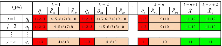
Generalized accelerations in the rotational differential equations: In Eq. (35), the expressions that encompass q_k, _kt and X_k can be represented as,

26

Fig. 2. Inertia matrix of the rotational motion equations in the flight phase

where j_k, j_k, jU_k, _k

j



, _k

j



, _k

j_U

, _k

j



, j_k, j



_ref and j



_ref are presented in Appendix. The constituent terms of Exp. (I), numbered from (1) to (12), form the inertia matrix of the rotational differential equations that illustrated in Fig. 2.

Coriolis and centrifugal forces in the rotational differential equations: In Eq. (35), if all the expressions that do not encompass generalized accelerations (q_k, _kt and X_k) are transferred to the RHS, one may obtain:

   

    

   

   



14 13

1

Re





 



        

 n

j i

i i

j T i i n

j i

i i

j T O i

q _{q q}

i

j T

ω

S r

(52)

where

i i i i i i v i i i i i O

i i i

i _{B B B B}

i

v ω ω ω

r

S ₀ 2 _{2 3 ,} ~ ₃

,   

   (53)





i

i i i i i v i i i i i i O

i i i

i _{B B B B B}

i

v ω ω ω

r

T ₃ 2 _{8 9 10 ,} ~ ₉

,    

   (54)

The constituent terms of Eq. (52), numbered (13) and (14), construct the RHS vector of the rotational differential equations that depicted in Fig. 3.

Generalized accelerations in the vibrational differential equations: In Eq. (36), all the expressions that encompass generalized accelerations (q_k, _kt and X_k) as their coefficients can be represented as,

Fig. 3. Right hand side of the rotational motion equations for the flight phase

 

q

I k1 k 2  kn kn1 kn2

1

q_ _{11 } _1m q_2 ₂₁  2m  qn n1  nm X1 X2

1



j q1 1+2+3 4+5+6+7+8+10 1+2+3 4+5+6+7+8+9+10 1+2 9+10 11+12 11+12

2



j q_2 1+2+3 4+5+6+7+8 1+2+3 4+5+6+7+8+10 1+2 9+10 11+12 11+12

 

n

j q_n 1+3 4+6+8 1+3 4+6+8 1 10 11 11

1

Req Req₂ .... Req_j ....

1

Re



n

q

Re

qn

T

 











,

27  n k n n k n k ref ref j T jf n n k n k ref ref j T jf n n k n k ref ref j T jf n n k n k ref ref j T jf kt n j k m t kt k j T jf n j k m t kt k j O O j T jf n j k m t kt k j T jf j k m t kt k j T jf n k m t kt k j T jf n k m

t k kt j T jf n k m

t k kt j T jf m t jft j k m

t k kt j T jf j k m

t k kt

j T jf n k m

t k kt

j T jf n k m

t k kt

j T jf n k m

t k kt

j T jf n k m

t k kt

j T jf n k m t kt k j T jf k j k k k k j T jf j k k k k j T jf n k k k k j T jf n k k k k j T jf n k k k k j T jf n k k k k j T jf n k k k k j T jf X R R R r R R C R W V U q R W V U x j k                                                                                                                                                          









 

 

 







































                                                                                                                                                             2 1 40 1 2 1 39 2 1 38 2 1 37 1 1 36 2 1 35 1 / 1 1 34 1 1 1 1 33 1 1 1 1 32 1 1 1 31 1 1 1 30 1 29 3 1 1 1 28 2 1 1 27 1 1 1 1 26 2 1 1 25 2 1 1 24 1 1 1 23 1 1 1 22 1 21 3 , 1 1 20 3 , 1 1 1 19 3 , 1 18 3 , 1 1 17 3 , 1 16 3 , 1 15 3 , 1 ~ X C X θ X θ X r α θ C θ C r r C r r r θ r θ θ α θ C θ r θ r θ θ θ θ θ θ x α x C x r x r x θ x θ θ              (II)

The constituent terms of Exp. (II), numbered from (15) to (40), establish the inertia matrix of the vibrational differential equations as illustrated in Fig. 4.

Fig. 4. Inertia matrix of the vibrational motion equations for the flight phase

 



I k 1 k 2  k n kn1 kn2

1

q_ ₁₁  1m q2 21  2m  qn n1  nm X1 X2

1



j

11

 15 +16 +17 +18 +19 +21 22+23+24+25+26 29+30+31+32 15 +16 +17 +18 +19 22+23+24+25+26 +30+31+32+34+36 15 +16 +18 34+35+36 37+38 39+40 37+38 39+40  m 1  2  j 21

 15 +16 +17 +18 +19 +20 +21 22+23+24+25+26 28+30+31+32+33 15 +16 +17 +18 +19 +21 22+23+24+25+26 29+30+31+32 15 +16 +18 34+35+36 37+38

39+40 37+38 39+40

 m 2    n j 1 n  20

+21 27+28+33 +2120 27+28+33 21 29

 40 40

28

Fig. 5. Right hand side of the vibrational motion equations for the flight phase

Coriolis and centrifugal forces in the vibrational differential equations: In Eq. (36), all the expressions that do not encompass the quasi-accelerations can be presented as,



    

  

 



    

  

 



43 1

42 1 41

Re



_{ }



_{ } 

   

    

 n

j

i i

i

jf T i i i

i n

j i

jf T O i

jf i

jf Q T

ω

S r

 



(55)

where

jf T

j v j jf T O j j j jf m

k

T j j jfk jk T

j j m

k jk jkf

jf K vj

Q 



_1  ω 



_1 C₄  ω  ω  r C₁  ω _, α

,

2    

 (56)

The constituent terms of Eq. (55), which are numbered from (41) to (43), form the RHS vector of the vibrational differential equations as demonstrated in Fig. 5.

Generalized accelerations in the translational differential equations: In Eq. (37), all the expressions that encompass q_k, _kt and X_k have been gathered as,

tot j n

kt n

k m

t

kt k ref T

n j ref n

k m

t

kt k ref T

n j ref n

k m

t

kt k ref T

n j ref

n

k m

t

kt k ref T

n j ref k

n

k

k k k ref T

n j ref n

k

k k k ref T

n j ref

X M V

R

q V

 

  



  

  



  

 



 

     

 

 

 



   

 

    

  

 

 

















  

   

  

   

  

   

  

   

   

    

   

    

   

50 1

1 1

49 2

1 1

48 1 1

47 1

1

1 1

46 1

45

3 , 1

1

44

3 ,

   

θ

X

θ

X C

X

r X

x X

x X

(III)

where refV_k , ref_k , ref_k , _k

ref_V

, _k

ref



and

M

tot are presented in the Appendix. The constituent

terms of Exp. (III), which are numbered from (44) to (50), form the inertia matrix of the translational differential equations as displayed in Fig. 6.

Fig. 6. Inertia matrix of the translational motion equations in the flight phase

11

Re_ .... Re_1m .... Rej1 .... Re_jm .... Re_n1 .... Re_nm

T

 

 



 ,

Re_ 41+42+43 .... 41+42+43 .... 41+42+43 .... 41+42+43 .... 41 .... 41

 



X

I k 1 k 2  k n kn1 kn2

1

q 11  1m q2 21  2m  qn n1  nm X1 X2

1

 n

j X_{1 +45}44 46+47+48+49 ₊₄₅44 46+47+48+49 45 47 50 0

2

 n

29

Fig. 7. Right hand side of the translational motion equations for the flight phase

Coriolis and centrifugal forces in the translational differential equations: In Eq. (37), all the expressions which do not encompass q_k, _kt and X_k can be represented as:

   

   



51 1

Re





     n

i

i i j T O i

X

X

i

j S

r

(57)

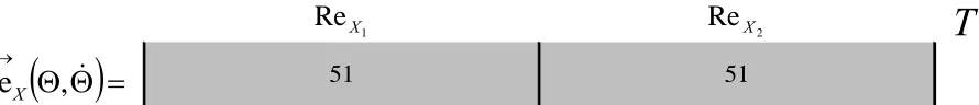
The constructive term of Eq. (57) which is numbered (51), form the RHS vector of the translational differential equations as exhibited in Fig. 7.

3.2.2. Assembling the inertia matrices and the RHS vectors of motion equations

In the previous section, the inertia matrices for the rotational (Fig. 2), vibrational (Fig. 4) and translational (Fig. 6) motion equations were obtained. By assembling these three matrices, the inertia matrix of the system obtains as shown in Fig. 8.

Fig. 8. Inertia matrix of the whole system in the flight phase

1

Re_X Re_X2

T

 











,

Re

_X 51 51

 



f

I k 1 k 2  k n kn1 kn2

1

q_ _{11 } _1m q_2 _{21 } _{2m } q_n n1  nm X1 X2

1



j

1

q_ I I I I I I I I

11



 II II II II II II II

m

1



2



j

2

q I I I I I I

21



 II II II II II

m

2



 

n j

n

q I I I I

1

n 

 II II II

nm 

1

 n

j X₁ III III

2

 n

30

Fig. 9. Right hand side vector of governing equations for the flight phase

The inertia matrix of this robotic system is symmetric. Therefore, in Fig. 8, it is sufficient to compute only those parts that are specified as (I), (II) and (III). This procedure is covered with details in the Appendix. Finally, by assembling the RHS vectors in the rotational (Fig. 3), vibrational (Fig. 5) and translational (Fig. 7) differential equations, Coriolis and centrifugal forces of the motion equations in the flight phase will be obtained as shown in Fig. 9.

3.3. Dynamics of the system in the impact phase

To accomplish the objectives of this section, the absolute velocity of each joint should be determined first. Apparently, for a serial manipulator constructed of n elastic links, there are

1



n joints and end points. The absolute velocities of these n1 points can be represented as,

 

 

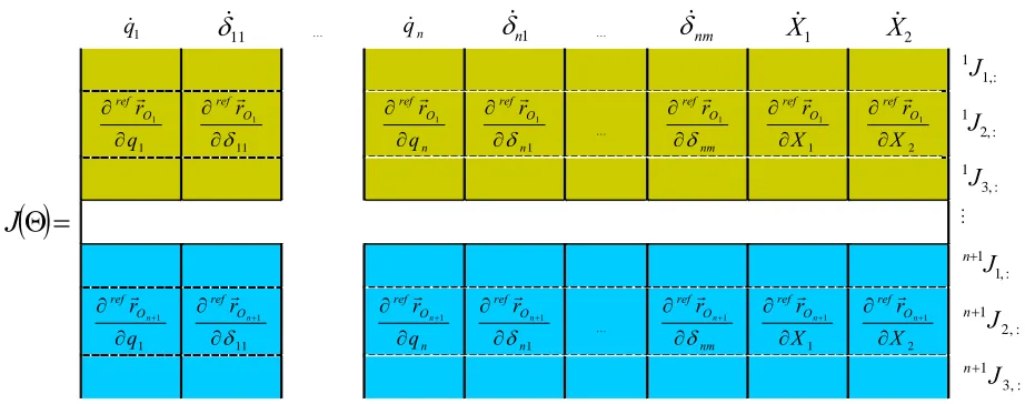
Θ r_   J  

i

O ref

, ₍₅₈₎

where J

 

 is the Jacobian matrix of the aforementioned robotic system which is illustrated in Fig. 10. It should be noted that O j

ref

i 

 r / is the derivative of the ith joint’s position with respect to the jth generalized coordinate. Also j_,:

i_J

represents the Jacobian matrix for the jth row ( j1....3) and every column (1....n2) of the ith joint (i1....n1).

An impact phenomenon happens when any joint or end point of the above-mentioned robotic system touches the ground. So, by considering Eq. (38), the system’s motion equations in the impact phase can be presented as,

Fig. 10. Jacobian matrix of n flying flexible links

1

q_ _{11 } _1m q_2 _{21 } _{2m } q_n n1  nm X1 X2

T

 

 





,

Re +14 13

41 +42 +43



41 +42 +43

13 +14

41 +42 +43



41 +42 +43

 14 41  41 51 51

1

q ₁₁  qn n1  _nm X₁ X₂

: , 1 1_J

1 1

q rO ref



 

11 1

  refrO

n O ref

q r

 

1



1 1

n O ref_r

 

 



nm O ref_r

  

1



1 1

X rO ref



 

2 1

X rO ref



 

: , 2 1_J

: , 3 1_J

 





J



: , 1 1_J

n

1 1

q rO_n ref

   _

11 1

   O_n

ref_r

n O ref

q r _n



 _

1



1 1

n O ref

n

r

    _



nm O ref

n

r

 

 _

1



1 1

X rO_n ref

   _

2 1

X rO_n ref

   _

: , 2 1_J

n

: , 3 1_J

31

 

 

J

   

t

I T

f  Θ Re,  



F (59)

where F

 

t indicates the applied forces exerting on the joints or end points during their collisions with the ground. By integrating Eq. (59) over the impact time (t t), we get:

 





 



 





 



 





 _



 

_

 



         

  

 Θ

F

Θ

F

Θ

Θ  T  _f 

f T

f J I J I

I (60)

where t

 

t dt

t





 F

F  and also, Θ/ Θ are the generalized velocities just before/after an impact. Eq. (60) presents n+nm+2 equations and n+nm+2+Number of Contact Points unknowns. The additional equations can be obtained by having the relationship between the pre- and post-impact velocities of joints or end points that collide with the ground, as follows:

 

_ _Θ _eJ

 

_ _Θ

J ₍₆₁₎

In above equation, which is called the Newton’s impact law, e denotes the coefficient of restitution. By combining Eqs. (60) and (61) and forming them in matrix format, we get

 

 

 

 

 



 



 



 

    

  

 

 

          

 

 _{ }

 

Θ

F

Θ _

 

 

 

 

 eJ

I J

J

I _f

I T f

i

0 ₍₆₂₎

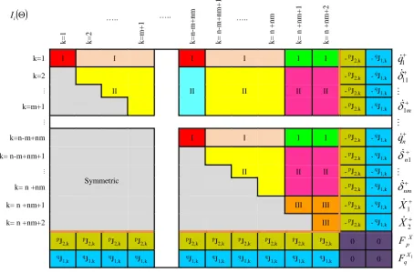
For example, if two impulsive forces of



FpX2

 

t and F

 

t X q 1



are respectively and

simultaneously exerted on the pth joint in the refX₂ direction and on the qth joint in the refX₁ direction, then two rows and columns should be incorporated to the initial inertia matrix obtained for the flying phase to establish the inertia matrix in the impact phase (see Fig. 11). Pre-multiplication of both sides in Eq. (62) by 1

 



i

I provides the unknown variables. The outcomes of the impact phase are the new initial conditions for the next flying phase.

4. Computer simulations

Here, the results of two computer simulations are presented to verify the proposed model.

Case study 1: For the first simulation, a planar single flexible link which is shown in Fig. 12, is simulated. This system is released with the following initial conditions.

; 0 ;

1 0 ;

0

; 5 . 0 ;

0 ;

0 ;

0

|

|

|

|

|

|

|

0 2 1 0

11 0

1

0 2 0

1 0

11 0

1

s m X

X s s

rad q

m X

m X

rad q

t t

t

t t

t t

 

 

 

 

 



 

 

  

 



32

Fig. 11. A sample inertia matrix of the impact phase

The elastic properties of this flexible link is modeled by the first eigen function of EBBT with clamped-clamped boundary conditions.



4.731



1.017cos



4.731



sinh



4.731



1.017cosh



4.731



sin

211    

x ₍₆₃₎

 

d dx

x₃11  211 ₍₆₄₎

Fig. 12. A single flexible link released from a specific height

 



i

I

k=

1

k=

2

…..

k=

m+

1

…..

k=

n-m+

nm

k=

n

-m+

nm+

1

…..

k=

n

+

n

m

k=

n

+

n

m+

1

k=

n

+

n

m+

2

k=1 I I I I I I - pJ2,k - qJ1,k q₁

k=2 - pJ2,k - qJ1,k



11 

 II II II II II - pJ2,k - qJ1,k 

k=m+1 - pJ2,k - qJ1,k



m

1 

 _

k=n-m+nm I I I I - pJ2,k - qJ1,k



n q_

k= n-m+nm+1 - pJ2,k - qJ1,k



1

n





Symmetric

II II II - pJ2,k - qJ1,k 

k= n +nm - p_J

2,k - qJ1,k



nm



k= n +nm+1 III III - pJ2,k - qJ1,k



1

X

k= n +nm+2 III - pJ2,k - qJ1,k



2

X

p

J2,k pJ2,k pJ2,k pJ2,k pJ2,k pJ2,k pJ2,k pJ2,k pJ2,k pJ2,k 0 0 2 X p

F

q

J1,k qJ1,k qJ1,k qJ1,k qJ1,k qJ1,k qJ1,k qJ1,k qJ1,k qJ1,k 0 0

1

X q

F

1

O O2

Surface Rigid

1

X

ref

2

X

ref x_1,1

2 , 1

x

2

X

j

1



1

X

2

X

Link Flexible

1

q_

g



1

33

Table 1. Required parameters for simulating the planar motion of a single flexible flying link

Parameters Value Unit

Length of the link l11 m

Mass per unit length ₁1 kg ∙ m

Bending stiffness 1000

3 

x

EI N ∙ m

Mass moment of inertia per unit length 1 10 5

94 . 2 0 0

0 94 . 2 0

0 0 89 . 5

    

 

  

  

J kg ∙ m

Gravity g9.81 m ∙ s

Coefficient of restitution e1

The necessary parameters for the simulation can be found in Table 1. Also, the results of the numerical solutions are depicted in Figs. 13-20.

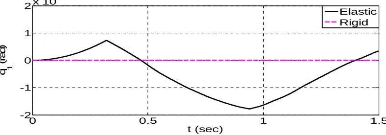
Fig. 13. Angular position of the flexible link

Fig. 14. Angular velocity of the flexible link

0 0.5 1 1.5

-2 -1 0 1 2x 10

-15

t (sec)

q 1

(ra

d

)

Elastic Rigid

0 0.5 1 1.5

-1.5 -1 -0.5 0 0.5 1 1.5x 10

-14

t (sec)

d

q 1

/d

t

(ra

d/

se

c

)

34

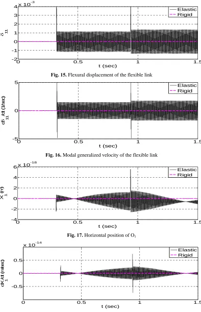
Fig. 15. Flexural displacement of the flexible link

Fig. 16. Modal generalized velocity of the flexible link

Fig. 17. Horizontal position of O1

Fig. 18. Absolute velocity of O1 in the refX1 direction

0 0.5 1 1.5

-2 -1 0 1 2 3 4x 10

-3

t (sec)

 11

Elastic Rigid

0 0.5 1 1.5

-5 0 5

t (sec)

d

 11

/d

t (

1

/s

e

c

)

Elastic Rigid

0 0.5 1 1.5

-4 -2 0 2 4 6x 10

-18

t (sec)

X 1

(

m

)

Elastic Rigid

0 0.5 1 1.5

-0.5 0 0.5

x 10-14

t (sec)

d

X 1

/d

t (

m

/s

e

c

)

35

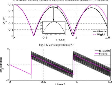
Fig. 19. Vertical position of O1

Fig. 20. Absolute velocity of O1 in the refX2 direction

The simulation results indicate that the system collides with the rigid surface at two different times: t0.3194sec and t0.9388 sec. The flexible link has almost no rotational motion. This fact can be concluded from Fig. 13 and Fig. 14. Also, the horizontal motion of this elastic link is negligible according to Fig. 17 and Fig. 18. Fig. 19 indicates that when the link is assumed rigid, it will reach its initial height (X₂ 0.5m), based on the conservation of energy law. When the link is assumed flexible, it will not reach its initial position. This is predictable; because when the elastic link strikes the ground, part of its energy will be converted to vibration energy due to the excitation of vibrational modes.

Case study 2:The purpose of the second case study is to compare the computational complexity of the algorithm proposed in the current paper with the method presented in [37]. A two-flexible-link planar robotic manipulator confined within a circle is simulated for this purpose. The computer simulation results of this model can be found in Figs. 12-20 of [37]. As expected, the same results are obtained by the developed algorithm proposed in the current work. To save space, the time responses of this system have not been presented in the current paper. However, the computational procedures required to obtain the governing equations of the aforementioned robotic systems by both recursive algorithms are presented in Table 2. In general, the required number of mathematical operations of 3×3 rotational matrices is less than that of 4×4 transformation matrices. For example, the CPU time for deriving the motion equations of this two-link flexible robotic system taken by the Intel (R) Core (TM) i3-3220 processor running at 3.3 GHz is 17.96sec for the 3×3 rotational matrices and 21.13 sec for the 4×4 transformation matrices respectively.

0 0.5 1 1.5

0 0.1 0.2 0.3 0.4 0.5

t (sec)

X 2

(

m

)

Elastic Rigid

0.55 0.6 0.65 0.7 0.75 0.4

0.42 0.44 0.46

0 0.5 1 1.5

-5 0 5

t (sec)

d

X 2

/d

t (

m

/s

e

c

)

36

Table 2: Required mathematical operations for recursive algorithms based on

3×3 rotational matrices and 4×4 transformation matrices

Sums Products Method

2 2 2

2 2

2

5 3 15

11

4 13

6 26 18

n m n m n

m

mn mn

m n

  



 

  

2 2 2

2 2

2

2 9 3 2

45 2

33

6 18

9 2 75 27

n m n m n

m

mn mn

m n

  



 

  

3×3

2 2 2

2 2

2

4 6 28

20

9 25

10 48 33

n m n m n

m

mn mn

m n

  



 

  

2 2

2 2

2

2

2 15 6

2 75 2

55

10 27

13 2

125 41

n m

n m