Please cite this article in press as: Abadi A, Pahlavanzade B, Zayeri F, Baghfalaki T. Interpretation of exposure effect in competing risks Original Article
Interpretation of exposure effect in competing risks setting under accelerated failure time models
Alireza Abadi1, Bagher Pahlavanzade2*, Farid Zayeri2, Taban Baghfalaki3
1 Department of Community Medicine, Faculty of Medicine, Shahid Beheshti University of Medical Sciences, Tehran, Iran 2 Department of Biostatistics, School of Allied Medical Sciences, Shahid Beheshti University of Medical Sciences, Tehran,
Iran
3 Departments of Statistics, Faculty of Mathematical Sciences, Tarbiat Modares University, Tehran, Iran
ARTICLE INFO ABSTRACT
Received 14.07.2017 Revised 09.09.2017 Accepted 08.12.2017
Background & Aim: In survival studies, incidence of competing risks causes that the time of event of interest to be unknown. Analysis of competing risk data, often implemented using hazard-based method under proportional hazard assumption. In this study, we interpreted covariate effect under accelerated failure time model and cause-specific survival function. Methods & Materials: We considered Weibull hazard and survival function as cause-specific hazard and survival function and explored the relation between these function. Estimation of parameters performed using Bayesian methods with non-informative priors that implemented in R2WinBUGS package of R software.
Results: Simulation study showed that, the relation between hazard and survival parameters for Weibull distribution is also established between parameters of cause-specific hazard and cause-specific survival function. This relation also verified in PBC data set for logarithm of serum bilirubin and D-penicillamine effect.
Conclusion: Although in competing risk studies, most of the analysis performed under PH assumption, analysis based on AFT models will also be applicable for these data. In these setting, coefficients can be interpreted as effects of covariate on time to each event. Key words:
Competing risk; Cause-specific hazard; Cause-specific survival; Weibull;
Accelerated failure time model
Introduction
In many survival studies, the risk of interest cannot occur due to incidence of another risk. These other causes are considered as competing risks of the event of interest. Incidence of competing risks causes the time of incidence of the event of interest to be unknown. For example, in a cancer study investigating the time from treatment initiation to cancer-related death, deaths from cardiovascular diseases are competing events. In most applications of competing risks, one risk considered as risk of interest, while other risks can be classified to one group and considered as competing risks (1-3).
Analysis of competing risks data is performed under two approaches including latent failure
times and bivariate approach. In the latent failure times approach, it is assumed that for each of the K potential events of D1, …, DK, there is a
potential failure time variable X1,X2,…,XK or
latent failure time. However, only their minimum
value i.e. = min ( , , … , ) can be
observed. In this approach, because for each individual only one of the X’s i.e. Xk is observable
then the correlation between the X’s cannot be estimated from observed data that lead to unpopularity of this approach (2, 4).
In the bivariate approach, instead of K potential time variables of X1,X2,…,Xk, variable
T considered as the event time and variable d that indicate type of event. These two variables (T,d) are modeled concurrently. In this approach, there are several methods of analysis including mixture models, vertical modeling, regression based on
pseudo-observations, Fully Specified
Subdistribution model, as well as models based on hazard function, which itself includes Cause-_____________________________________________________
92
specific hazard regression and Subdistribution hazard regression. Methods based on hazard function are commonly used for analyzing competing risk data. In bivariate approach, there is no need to assumption about independence of competing risks (1,2,5).
Application of cause-specific hazards function under both PH and AFT assumptions was first proposed by Prentice (6). In this method, to estimate the parameters of each event, the events from other causes are considered as censored and estimation of parameters under PH assumption is interpreted as probability for failing from an event of type k in an infinitesimal small time interval given that he/she has not experienced any of the events so far. In addition to cause-specific hazard function, Prentice and Kalbfleich proposed cumulative incidence function which indicates the cumulative probability of incidence of the event of interest in the presence of competing risks (3,7).
In cause-specific models, cumulative incidence function for each event is a function of cause-specific hazard of all events. As in this method the effect of exploratory variable on competing events is not considered, thus the resulting estimations cannot be directly translated to a higher effect of variable on incidence of the event of interest. In other words, a higher cause-specific hazard for event k for one group does not necessarily transform to a higher cumulative incidence of that event for that group (3,7). To estimate the effect of exploratory variables on the cumulative incidence of each risk, fine and gray proposed sub-distribution hazards function, in which there is a direct relationship between estimation of parameters of the risk function and the cumulative incidence function(8). Modeling of CIF (Cumulative incidence function) by parametric distributions through direct and indirect methods was proposed by Jeong (7,9).
If parametric distribution provides a good fit to survival time, parametric models would be more efficient than nonparametric and semi-parametric methods because in these methods fewer parameters need to be estimated (10). Under the cause-specific hazard method, parametric distributions have mainly used for modeling of CIF (7, 9-11). Parametric distributions have also been used in mixture models (12-14) . Parametric distributions have been investigated for analyzing competing risks under the latent failure time approach by both ML and Bayesian methods.
Firstly, Basu and Klein used Weibull and exponential distributions under PH assumption and ML estimation method (15-17). DeGroot and Goul also used Bayesian methods for estimation of exponential distribution parameters in ALT models (18). Tan (19), Benue and Mazuchi et al (20) as well as Xu et al (21) employed Weibull and exponential distributions in ALT models using Bayesian methods for estimation of parameters.
Under PH assumption, parameters interpreted as relative risk of incidence event and in models under AFT assumption, interpretation of risk factors is performed on survival time (failure time). In other words, in these models, the logarithm of survival time is modeled as a function of exploratory variables (22).
One of the parametric distributions widely used in survival analyses is Weibull distribution. The unique feature of this distribution is that if PH assumption holds then AFT assumption also holds, and also there is a relation between estimation of parameters under the two models (23).
In competing risks settings, if we are looking for etiology of disease, cause-specific competing risks models should be utilized. In these studies, due to the characteristics of the hazard function and flexibility of semi-parametric models, hazard-based regression methods are often expended under PH assumption and parametric models which often have AFT characteristics have attracted less attention. On the other hand, in competing risks analyses conducted by considering AFT assumption under different approaches, no interpretation has been presented for estimations of parameters based on the time until incidence of the event. Therefore, in this study we are after examining the relationship between regression coefficients of cause-specific hazard and cause-specific survival for Weibull distribution. We also want to check whether PH and AFT assumptions hold true for each of the risks. Based on these, we try to present a suitable interpretation of the effect of exploratory variables on the time until incidence of event in competing risks studies under AFT approach.
Methods
Cause- specific hazards models
λ ; ( ) = lim
→ ℎ ( ≤ < + ℎ, = |
≥ , ( ))
In this relation, λ ; ( ) is the rate of instantaneous incidence of the event type k at the time t in the presence of other competing risk. If events considered as mutually exclusive, then the overall hazard at each time is equal to the sum of all cause- specific hazards.
In the cause-specific hazard, the cumulative incidence is a function of cause-specific hazard of all events, which is defined as the following relation:
( | ) = ( | )exp − Λ ( | )
The likelihood function of the model of cause-specific competing hazards in the presence of K competing risks is:
= ( ; ( )) − ( ; ( )
Where, the first component indicates the risk function, while the second component represents the survival function, denotes the type of event. For Weibull distribution under PH assumption, in the above likelihood function, hazard and survival
functions replaced by ℎ ( ) =
and ( ) = exp(− ), respectively. In these functions is the scale parameter and p represents the shape parameter. To investigate the effect of exploratory variable, the scale parameter is often modeled asλ = exp ( + ).
In accelerated failure time models, the logarithm of the time variable is considered as a function of exploratory variables. When there is one exploratory variable, this model will be:
log( ) = + ∗ +
In which, is a random variable. If has a extreme value distribution, then log (Ti) will have Weibull distribution. In this case, the risk function and survival function will be:
ℎ( | ) = ℎ (log( ) − ( )/ ) ( | ) = (log( ) − ( )/ )
Where, ( ) is a function of exploratory
variables as ( ) = + ∗ . (. ) and
ℎ (. ) are the survival function and risk function of the extreme value distribution.
As can be seen in log-linear form of AFT models, a direct relationship is assumed between exploratory variables and the failure time variable. This means that in these models estimation of parameters can be interpreted based
on the effect of exploratory variable on the rate of progression of disease.
In standard survival studies, there is a relation between coefficients obtained from the PH and AFT forms of the Weibull models such that = − ∗ , in which β is the parameter estimation under PH assumption and α is the parameter estimation under AFT assumption, and p is the shape parameter. For example, when considering a binary exploratory variable, indicates that the risk of incidence of event in the exposure group exp(β ) time the risk of incidence in the group without exposure. Under PH assumption, this proportion remains constant over time. In contrast, shows that for all fixed value of survival probability S(t)=q, survival time in the exposure group (γ ) time the survival time in the group without exposure, and under AFT assumption, this proportion remains constant over time.
In this study, parameters estimated under Bayesian approach. Survival time assumed to follow Weibull distribution. Parameters were estimated under both PH and AFT assumptions. In Bayesian inference, for regression parameters, normal prior distribution N(0,0.01), and for parameter of shape (p), gamma distribution ~ (0.01,0.01) were considered. Model implemented in R2WinBUGS package of R software. The values of Gelman-Rubin statistics
close to 1 were considered as index for parameters convergence.
Results
The results of simulation study
First, the relationship between parameters of Weibull model under PH and AFT assumptions was examined by the simulation. In the simulations, two competing risks were considered independent of each other. Because for two independent variables with ~ ( , ) and
~ ( , ) distributions, variable T,
T=min(T1,T2) has Weibull distribution with the parameter form and the scale parameter λ = ( + ) / (25-27), thus time of event
of these two competing risks T was generated from ~ ( , ) distribution, and using Bayersman approach (4), it was allocated to two competing risks. Scale parameters were modeled as exponential functions of the form =
exp ( + ) and = exp ( + ) ,
94
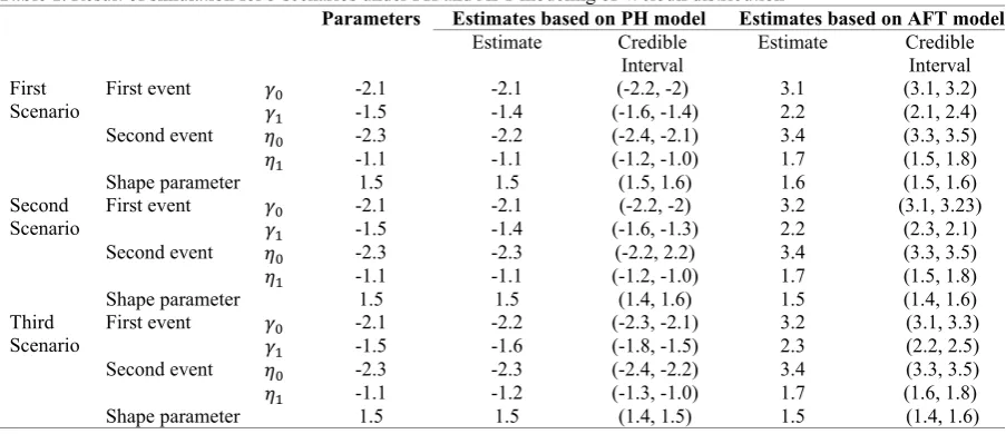
~ (1,0.5) distribution. Simulations were performed under three scenarios. The first scenario was considered without censoring. The second and third scenarios were performed with 5 and 10% censorship, respectively. The data of time until censorship was also generated from uniform distribution. All simulations are conducted with n= 100 and replicates 1000, with the results presented in table and diagram. The parameters of two risks were considered to be close to each other, so that the ratio of incidence of event out of each of the risks becomes close to 50%. These parameters are provided in the Table 1.
Comparison of estimations under PH model and real values demonstrate that the estimations are close to the real values of the parameters. By comparing the estimations under the three scenarios, it was observed that with increasing censoring level, estimation of the treatment parameter is more affected than other parameters. Comparison of the estimations of parameters under AFT assumption with the values obtained from β = − ∗ across all three scenarios
indicates that these two values are almost the same. In other words, between the parameters of cause-specific hazard and cause-specific survival, the relation β = − ∗ holds. Plots of cause-specific hazard and survival under both PH and AFT assumption for first scenario presented in Figures 1 and 2. The corresponding plots under the two modeling were completely similar. Based on the former, it is observed that the hazard of incidence in the treatment group (trt=1) is proportional to hazard in control group (trt=0) over time, where this ratio for the first event was exp(−1.4) = 0.24, and for the second event it was exp(−1.1) = 0.33. In the cause-specific survival plots, the survival probability of both treatment and control groups over time was proportional, and AFT assumption holds in each of the cause-specific functions. This means that for any value of survival probability S(t)=q, the ratio of time until the first event in treatment group to control group was exp(2.2) = 9.02, and the ratio of time until incidence of the second event in the treatment group to control group was exp(1.7) = 5.47.
Table 1. Result of simulation for 3 scenarios under PH and AFT modeling of Weibull distribution
Parameters Estimates based on PH model Estimates based on AFT model
Estimate Credible
Interval
Estimate Credible
Interval First
Scenario
First event -2.1 -2.1 (-2.2, -2) 3.1 (3.1, 3.2)
-1.5 -1.4 (-1.6, -1.4) 2.2 (2.1, 2.4)
Second event -2.3 -2.2 (-2.4, -2.1) 3.4 (3.3, 3.5)
-1.1 -1.1 (-1.2, -1.0) 1.7 (1.5, 1.8)
Shape parameter 1.5 1.5 (1.5, 1.6) 1.6 (1.5, 1.6)
Second Scenario
First event -2.1 -2.1 (-2.2, -2) 3.2 (3.1, 3.23)
-1.5 -1.4 (-1.6, -1.3) 2.2 (2.3, 2.1)
Second event -2.3 -2.3 (-2.2, 2.2) 3.4 (3.3, 3.5)
-1.1 -1.1 (-1.2, -1.0) 1.7 (1.5, 1.8)
Shape parameter 1.5 1.5 (1.4, 1.6) 1.5 (1.4, 1.6)
Third
Scenario First event -2.1 -1.5 -2.2-1.6 (-2.3, -2.1) (-1.8, -1.5) 3.22.3 (3.1, 3.3) (2.2, 2.5)
Second event -2.3 -2.3 (-2.4, -2.2) 3.4 (3.3, 3.5)
-1.1 -1.2 (-1.3, -1.0) 1.7 (1.6, 1.8)
Shape parameter 1.5 1.5 (1.4, 1.5) 1.5 (1.4, 1.6)
Application in real data
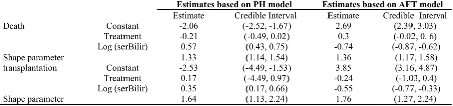
To apply the model in real data, data of PBC study was used. These data are also available in JM package of R software. In this study, 312 patients suffering from biliary cirrhosis participated, where 158 and 154 individuals received medication and placebo, respectively. The main objective of PBC study was to investigate the effect of intake of D-penicillamine on survival of patients. For this purpose, in addition to the information associated with basic variables including age at the beginning of the study, gender, etc. follow-up information of markers such as serum bilirubin has also been registered. In this dataset, for survival variable Weibull distribution has been used in other studies (24). In this study, death has been considered as the first event and receiving transplant has been regarded as the second event. Further, the effect of the value of serum bilirubin at the beginning of the study on the risk of incidence of each of the two events was examined under PH modeling. Also, the effect of this marker on the duration until incidence of each of the two events was investigated under AFT modeling after controlling the effect of receiving treatment. Out of the 312 patients in the study, 140 died and 29 received a transplant. Shape parameter for either of the two events was considered unique. The results of model fitting
under PH and AFT modeling have been reported in the Table 2.
As can be seen from the above table, estimation of treatment effect under PH model was obtained as -0.21 for death and 0.17 for transplantation. However, the credible interval for both parameters involved value of zero. In other words, the risk of incidence of death event as well as the risk of transplantation was not significantly different among treatment and control group. Estimation of these parameters under AFT model was obtained as 0.3 and -0.24 for death and transplantation, respectively. Here also the credible interval involved the value of zero for both parameters. In other words, the time until death and transplantation has not significantly different among the individuals in the treatment and control groups. Under PH assumption, estimation of the parameter of logarithm of serum bilirubin variable was obtained as 0.57 and 0.35 for death and transplantation, respectively. Under AFT assumption, estimation of the logarithm of serum bilirubin variable parameter was obtained as -0.74 and -0.55 for death and transplantation, respectively.
By comparing estimation of parameters under AFT model with the values obtained from β = − ∗ , it is observed that the obtained values are very close to each other. For example, estimation of logarithm of serum bilirubin parameter under AFT model (-0.74) and the value obtained from Figure 2. Cause-specific survival plot for first scenario of simulation
Table 2. Result of cause-specific modeling under PH and AFT assumption for PBC data
Estimates based on PH model Estimates based on AFT model Estimate Credible Interval Estimate Credible Interval
Death Constant -2.06 (-2.52, -1.67) 2.69 (2.39, 3.03)
Treatment -0.21 (-0.49, 0.02) 0.3 (-0.02, 0. 6)
Log (serBilir) 0.57 (0.43, 0.75) -0.74 (-0.87, -0.62)
Shape parameter 1.33 (1.14, 1.54) 1.36 (1.17, 1.58)
transplantation Constant -2.53 (-4.49, -1.53) 3.85 (3.16, 4.87)
Treatment 0.17 (-4.49, 0.97) -0.24 (-1.03, 0.4)
Log (serBilir) 0.35 (0.17, 0.66) -0.55 (-0.77, -0.33)
96
β = −γ ∗ = −0.75 are very close to each other. Further, estimation of the parameter of this variable for transplantation event under AFT model was obtained as -0.55, which is very close to β = − ∗ = −0.57. For the group therapy variable, it is also observed that under AFT assumption, estimation of treatment parameter was obtained as 0.3 and -0.24 for the event of death and transplantation, respectively. Estimation of parameters using β = −γ ∗ gave 0.28 and -0.28, respectively. Estimation of shape parameter under PH model was obtained as 1.33 and 1.64 for death and transplantation, respectively. The values of estimation of this parameter under AFT model for both events were obtained to be slightly higher than those obtained by PH model, obtained as 1.36 and 1.76 for death and transplantation, respectively.
Discussion
In competing risks studies conducted in the area of medical sciences, mostly hazard-based models, i.e. cause-specific hazards and sub-distribution hazards methods are used. This is because, in this approach the analysis can be performed without identifiability problems and all measures can be estimated from observable data. Most studies conducted on hazard-based models have been performed under the assumption of proportionality of hazards (PH) and using semi-parametric methods (1). On the other hand, performing analyses under AFT assumption by parametric or semi-parametric methods has been draw less attention. Even in case of application of these models, no interpretation has been presented regarding the effect of exploratory variable on the time until incidence of the events (7, 12-14, 25-27). In this study, at first the relationship between estimation of parameters of cause-specific hazard function and survival function of Weibull distribution was examined and then interpretation of the estimations of parameters under AFT Weibull model presented. The simulations indicated that under Weibull distribution, if PH assumption holds in the cause-specific hazard function, it can be concluded that AFT assumption also holds in cause-specific survival function. For each of the risks, β = − ∗ holds between the parameters of cause-specific hazard function and cause-cause-specific survival function. Next, cause-specific hazard and cause-specific survival analysis was performed
for PBC data under Weibull distribution. It was observed that the relation is also applicable in these dataset. The difference observed in
parameter estimation associated with
transplantation event can be a result of the small number of this event.
in the logarithm of serum bilirubin, the time until incidence of death event decreases by exp(−0.74) = .47 times, and time until transplantation is shortened by exp(−0.55) = .57 times. Comparing these two interpretations, it can be said that in the patients suffering from biliary cirrhosis, each unit reduction in the logarithm of serum bilirubin increases the time until death and transplantation by (1/0.47)= 2.12 and (1/0.57) = 1.57 times, respectively. In contrast, for each unit increase in the logarithm of serum bilirubin, the probability of death event at any short time interval increases by 1.76 times, and for transplantation, it grows by 1.41 times. It is observed that understanding the effect of variable under AFT assumption is easier.
Conclusion
The results of this study indicated that the relationship between coefficients of Weibull distribution under two modeling also holds true in cause-specific hazard models. It was also observed that if AFT assumption holds in cause-specific survival functions, interpretation of coefficients can be accomplished on the time until incidence of each of the events.
Acknowledgments
This article has been extracted from the thesis of Bagher Pahlavanzade in School of Allied Medical Sciences, Shahid Beheshti University of Medical Sciences. The authors wish to thanks the participants in the study and the Vice Chancellor of Research Affairs of Shahid Beheshti University of Medical Sciences for its financial support.
Conflict of Interest
The authors declare that they have no competing interests.
References
1. Haller B, Schmidt G, Ulm K. Applying competing risks regression models: an overview. Lifetime Data analys. 2013:1-26.
2. Haller B. The analysis of competing risks data with a focus on estimation of cause-specific and subdistribution hazard ratios from a mixture model: LMU; 2014.p.23-90.
3. Kalbfleisch JD, Prentice RL. The statistical analysis of failure time data: John Wiley & Sons; 2011.p.12-56.
4. Beyersmann J, Allignol A, Schumacher M. Competing risks and multistate models with R:
Springer Science & Business Media; 2011.p.110-6.
5. Klein JP, Van Houwelingen HC, Ibrahim JG, Scheike TH. Handbook of survival analysis: CRC Press; 2016.
6. Prentice RL, Kalbfleisch JD, Peterson Jr AV, Flournoy N, Farewell VT, Breslow NE. The analysis of failure times in the presence of competing risks. Biometrics. 1978:541-54. 7. Jeong JH, Fine J. Direct parametric inference for
the cumulative incidence function. Journal of the Royal Statistical Society: Series C (Applied Statistics). 2006;55(2):187-200.
8. Fine JP, Gray RJ. A proportional hazards model for the subdistribution of a competing risk. Journal of the American statistical association. 1999;94 (446):496-509.
9. Jeong JH. A new parametric family for modelling cumulative incidence functions: application to breast cancer data. Journal of the Royal Statistical Society: Series A (Statistics in Society). 2006;169(2):289-303.
10. Cheng Y. Modeling cumulative incidences of dementia and dementia-free death using a novel three-parameter logistic function. Int J Biostat. 2009;5(1).
11. Shayan Z, Ayatollahi S, Zare N. A parametric method for cumulative incidence modeling with a new four-parameter log-logistic distribution. Theoret Biol Med Model. 2011;8(1):43.
12. Lau B, Cole SR, Gange SJ. Parametric mixture models to evaluate and summarize hazard ratios in
the presence of competing risks with time‐
dependent hazards and delayed entry. Stat Med. 2011;30(6):654-65.
13. Lau B, Cole SR, Moore RD, Gange SJ. Evaluating competing adverse and beneficial outcomes using a mixture model. Stat Med. 2008;27(21):4313-27. 14. Dang UJ, McNicholas PD. Accelerated Failure
Time Models for Competing Risks in a Cluster Weighted Modelling Framework. arXiv preprint arXiv:1312.0859. 2013 Dec 3.
15. Klein JP, Basu AP. Weibull accelerated life tests when there are competing causes of failure. Commun Stat-Theory Methods. 1981;10(20): 2073-100.
16. Klein JP, Basu AP. Accelerated life testing under competing exponential failure distributions. Missouri Univ-Columbia Dept Statistics, 1981. 17. Klein JP, Basu AP. Accelerated life tests under
competing Weibull causes of failure. Commun Stat-Theory methods. 1982;11(20):2271-86. 18. DeGroot MH, Goel PK. Bayesian estimation and
optimal designs in partially accelerated life testing. Naval Res Logistics. 1979;26(2):223-35.
98
Maintainability and Safety, 2009 ICRMS 2009 8th International Conference on; 2009: IEEE.
20. Bunea C, Mazzuchi T. Competing failure modes in accelerated life testing. J Stat Plan Inference. 2006;136(5):1608-20.
21. Xu A, Tang Y. Objective Bayesian analysis of accelerated competing failure models under Type-I censoring. Comput Stat Data Analysis. 2011;55(10):2830-9.
22. Luo S. A Bayesian approach to joint analysis of multivariate longitudinal data and parametric
accelerated failure time. Stati Med.
2014;33(4):580-94.
23. Kleinbaum D, Klein M. Statistics for Biology and Health (survival analysis, ). New York: Springer-Verlag; 2005.p.65-89.
24. Rizopoulos D. Joint models for longitudinal and time-to-event data: With applications in R: CRC Press; 2012.p.11-45.
25. Benichou J, Gail MH. Estimates of absolute cause-specific risk in cohort studies. Biometrics. 1990:813-26.
26. Jiang R, editor Analysis of accelerated life test data involving two failure modes. Advanced Materials Research; 2011: Trans Tech Publ.p.23-90. 27. Tai BC, Machin D, White I, Gebski V. Competing
risks analysis of patients with osteosarcoma: a comparison of four different approaches. Stat Med. 2001;20(5):661-84.
28. Hyun S, Lee J, Sun Y. Proportional hazards model for competing risks data with missing cause of failure. J Stati Plan Inference. 2012;142(7):1767-79.