International Journal of Finance and Managerial Accounting, Vol.2, No.8, Winter 2017
19
With Cooperation of Islamic Azad University – UAE BranchFads Models with Markov Switching Hetroskedasticity:
decomposing Tehran Stock Exchange return into
Permanent and Transitory Components
Teymoor Mohammadi
Associate Professor, Faculty of Economics, Allameh Tabataba'i University, Tehran, Iran
Abdosade Neisi
Associate Professor, Faculty of Economics, Allameh Tabataba'i University, Tehran, Iran (Corresponding author)
Mehnoosh Abdollahmilani
Associate Professor, Faculty of Economics, Allameh Tabataba'i University, Tehran, Iran
Sahar Havaj
Ph.D. Candidate in Financial Economics, Faculty of Economics, Allameh Tabataba'i University, Iran
ABSTRACT
Stochastic behavior of stock returns is very important for investors and policy makers in the stock market. In this paper, the stochastic behavior of the return index of Tehran Stock Exchange (TEDPIX) is examined using unobserved component Markov switching model (UC-MS) for the 3/27/2010 until 8/3/2015 period. In this model, stock returns are decomposed into two components; a permanent component and a transitory component. This approach allows analyzing the impact of shocks of permanent and transitory components. The transitory component has a three-state Markov switching heteroscedasticity (low, medium, and high variances). Results show that the unobserved component Markov switching model is appropriate for this data. Low value of RCM criteria implies that the model can successfully distinguish among regimes. The aggregate autoregressive coefficients in the temporary component are about 0.4. The duration of high-variance regime for the transitory component is short-lived and reverts to normal levels quickly. The implied result of the research is that the presidential election may have a significant effect on being in the third regime.
Keywords:
1. Introduction
In the late 1970s, Fama et al. (1969) introduced the efficient market hypothesis. From their point of view, an efficient market adopts new sets of information quickly. Therefore, all price changes are unpredictable. In fact, efficient market prices always reflect all available information perfectly, and an investor cannot beat the market. According to this hypothesis, the best prediction for future prices is current prices. This process is known as a random walk process. In other words, this process does not have a memory, and expected returns are considered as constant. There are arguments against this hypothesis; one of those is the January Effect, which shows some predictable patterns for stock prices and questions the random walk behavior of the market prices. This was the most important anomaly phenomenon underlying the stock market crash in 1987.
The 1987 market crash, the sudden, up-and-down stock value of “dot-com” stocks, during the 1998-2000 periods, challenged traditional views of the efficient market hypothesis and introduced a new set of models called Fads models. These kinds of models are good substitutes for the random walk hypothesis mentioned above.
There is always a potential probability that prices may be far away from their fundamental values. This deviation from fundamental value exists because of speculative bubbles or Fads. In the stock market, the average of these deviations from fundamental value is caused by psychological and social powers like fashions in political views, consumption of goods, or something like ‘animal spirits’ in Keynesians (Shiller, 1984). Deviation from the fundamental value may occur in every market like car, food, house, etc. Shiller (1981) and Le Roy and Porter (1981) expressed that the observed deviations in stocks and bonds are high in corresponding markets and could not be explained by a set of available information in fundamental values (for example, dividends). To explain this additional deviation, Shiller focused on the role of overreacting investors, fashions, and fads in stock prices. In addition, West (1988) studied stock price fluctuations and concluded that the ‘rational bubble’ and other standard models did not explain stock price returns well, and thus introduced Fads models. Heteroscedasticity plays an important role in assessing and analyzing these kinds of models. Most studies in this field used Generalized Autoregressive Conditional
Heteroscedasticity (GARCH), which was considered as a suitable kind of model for stock markets. There are some problematic issues in this kind of heteroscedasticity model (Camerer, 1989). GARCH models imply an over-persistency in fluctuations, whereas, in time series data, there exist jumps, which GARCH models cannot explain. By solving the problem, Hamilton and Susmel (1994) assumed that big shocks in stock markets (like the 1987 crash in the U.S. stock market) might be the result of different existing regimes and switching between regimes controlled by a Markov chain pattern. They claimed that Switching Autoregressive Conditional Heteroscedasticity (SWARCH) explained the 1987 crash much better. In addition, in this field, Kim and Kim (1996) analyzed the U.S. stock market. Their study was focused on the 1987 crash. Their analysis used a fads model with Markov switching heteroscedasticity in both the fundamental value and the transitory component.
The goal of this study is to decompose Tehran Stock Market returns into fundamental values and fads components, using fads model and Markov switching heteroscedasticity. The rest of this paper is organized as follows: In section 2, the review of literature will be presented. In section 3, model specification and Gibbs sampling will be reviewed. Section 4 shows a summary of statistical data and empirical results. Eventually, Section 5 presents concluding remarks.
2. Literature Review
For investors, studying statistical characteristics of the financial series is crucial in this regard. The main question in this field is how do fluctuations of stock prices (or returns) behave? The U.S. stock market crash in 1987 challenged traditional efficient market hypotheses. This was an introduction for the appearance of fads models. In fact, fads models are a special form of unobserved-components model, introduced by Summers (1986) and Poterba and Summer (1988).
other words, conditional variances can jump; however, for capturing these jumps, GARCH models alone are not suitable for financial time series. Friedman and Laibson (1989) showed that it is not appropriate to use the same GARCH model to describe the consequence of both large and small shocks. Then, the usual constant-parameter GARCH specifications exhibit a poor statistical description of extremely large shocks. Many studies introduced new ways to solve the problem and caught some of those fluctuations, which variance ratio tests were not able to assess (for instance, Summers (1986), Campbell and Mankiw (1987), Kim, Nelson, and Startz (1991), Poterba and Summers (1988), Engle and Lee (1992), and Hamilton and Susmel (1994). In this regard, Hamilton and Susmel (1994) provided evidence that the possibility of extremely large shocks during the 1987 crash came from one of the several different regimes, with transition between regimes governed by an unobserved Markov chain. Beside, Kim and Kim (1995) examined the possibility that the 1987 stock market crash was an example of very large transitory shocks that are short-lived. Their paper employed a version of an unobserved component model with Markov-switching heteroscedasticity (UC-MS model).
The U.S market crash in 1987 was unusual from different aspects. This crash was the biggest one in indexes; only in one day, there was such a crash, unprecedented from 1885, and it suddenly increased stock price fluctuations. Later, Schwert (1990) showed that fluctuations came back to a lower level than previously predicted. Some studies confirmed Schwert’s results. For example, Engle and Chowdhury (1992) showed that persistency in fluctuations after the crash was weaker and implied there exist temporary structural changes in GARCH parameters. For a better explanation of stock price fluctuations after the 1987 crash, Engle and Lee (1992) decomposed stock prices into trend and transitory components and compared the results with the GARCH model. In this field, Kim and Kim (1996) expressed that the 1987 crash in the U.S. stock market may be a short-lived fads. After the crash, the stock market was again faced with another crash in ‘dot-com’ stocks during 1998-2001. There was a dramatic rise and a sudden fall. These fluctuations challenged the traditional view, which says stock price movements are always adjusted with a new set of information about fundamental values (Schaller and Van Norden, 2002).
In fact, in comparison with GARCH models, unobserved component models (UC models) with Markov switching consider more dynamic in stock market fluctuations. In addition, despite GARCH models, the level of fluctuation in these models comes back to the normal level rapidly. Heteroscedasticity may exist in state space models, particularly UC models. There are two possible kinds of heteroscedasticity: ARCH type conditional and Markov switching heteroscedasticity. They are fundamentally different but it may be difficult to distinguish between them. The conditional variance under ARCH is constant but subject to sudden shifts under Markov switching heteroscedasticity. In addition, long run dynamics of variances may be controlled by Markov switching (or regime shifts) in unconditional variance. Short run dynamics of variances may be an ARCH type heteroscedasticity within a regime. Therefore, Markov switching heteroscedasticity may be appropriate for low-frequency time series data over a long period, whilst ARCH type heteroscedasticity may be suitable for high frequency time series data over a short period (Kim and Nelson, 1999). Most studies in this regard suggest that a failure to allow changing in regimes leads to an over-persistence in variances of a time series, and it is possible to face an integrated ARCH or GARCH (Diebold, 1986; Lastrapes, 1989; Lamoureux and Lastrapes, 1990). An appropriate substitution for state space models with ARCH type heteroscedasticity is state space models with Markov switching heteroscedasticity.
The model used in this paper was first introduced by Summers (1986), and Poterba and Summers (1988). This model is often referred to as a ‘fads’ model (a particular form of ‘Unobserved component’ model):
(1)
(2)
(3)
Where is the natural log of stock price, is the fundamental value of stock prices evolving slowly over time, and is transitory component. The return, defined as a log-differenced price, is written as:
The transitory component has a root close, but not equal, to unity.
Many studies have introduced different methods for decomposing a univariate series into permanent and transitory components. For instance, Watson (1986) and Clark (1987) decomposed GNP into two components, using unobserved component (UC) models. Najarzadeh, Sahabi, and Soleimani (2013) decomposed inflation rate into permanent and temporary components, assessing the relationship between inflation and inflation uncertainty in long and short horizons. Alternative methods have been used for detecting mean reversion or fads in stock prices but none of them considers the possibility of very unusual and temporary deviations of stock prices from the random walk component (see, for example, Fama and French, 1988; Poterba and Summers, 1988; Lo and Mackinlay 1988; Kim, Nelson, and Startz, 1991; Kim, Nelson, and Startz, 1998).
Fama and French (1988) studied stock prices using a mean-reversion model (AR(1) autocorrelation) for the 1926-1985 data set. They represented the natural log of stock prices as a sum of a random walk process and a stationary process. Their main idea was that stock prices have a stationary process and the shocks of stock prices are composed of permanent and transitory shocks, which later will be decaying gradually. Results showed that autocorrelation coefficients have a U-shape pattern against the time horizon. These become negative for 2-year returns, reach minimum value for 3-4-year returns, and then move back toward zero for longer return horizons.
Kim and Nelson (1998) assessed Fama and French’s (1988) model for the 1926-1995 periods, again. They expressed that depression and years of war clearly apply a strong influence in the results but it is not clear whether the large returns of that period chip in information in the data or are rather a source of noise to be eliminated in estimates. They used a Gibbs sampling method for solving the heteroscedasticity problem. A test of structural change was applied and significant differences between pre- and post-war periods were suggested.
Hamilton and Susmel (1994) expressed that ARCH models often represent high persistency to stock volatility and have relatively poor forecasts. A good explanation for extremely high shocks (like the 1987 crash) was introduced as a Markov-Switching ARCH (SWARCH) model in their study. They
considered three different regimes in stock volatility: low, moderate, and high, which typically last for several years. A high-variance regime is related to the depression period. Their results showed that SWARCH specification offers better statistical fit to the data as well as better forecasts.
Kim and Kim (1996) examined the possibility that the 1987 stock market crash was a short-lived fad. They used a fads model with Markov-switching heteroscedasticity in both the fundamental and transitory components (UC-MS model). Although they usually thought of fads as speculative bubbles, what UC-MS model considers is unwarranted pessimism, shown by the market to the OPEC oil shock and the 1987 crash. In addition, the conditional variance implied by the UC-MS model captures most of the dynamic in the GARCH specification of stock return volatility. Yet, unlike the GARCH measure of volatility, the UC-MS measure of volatility is consistent with reverting to its normal level very quickly after the crash. Furthermore, this model can capture some short-run dynamics that may not otherwise be captured by variance ratio test, autoregression test or by conventional unobserved-component models. Aforementioned models may miss some important short-run dynamic of interest such as the 1987 crash because they do not explicitly address the importance of heteroscedasticity.
Hammoudeh and Choi (2004) studied Gulf Cooperation Council’s (GCC) stock markets. They used fads model with Markov switching heteroscedasticity both in fundamental and fads components, and came to two different regimes in two components. The GCC stock markets vary in terms of sensitivity to the magnitude of return volatility and the duration of volatility, regardless of the volatility regime and the return component.
variation in the duration of volatility states of the transitory component in market returns.
Chen and Shen (2012) examined the stochastic behavior of the returns on real estate investment trust (REITs) using unobserved component Markov switching (US-MS) model. In this model, REIT returns decomposed into permanent and transitory components with Markov switching heteroscedasticity in both components. The empirical evidence showed that, for all REIT returns, the overall variance of the transitory component is significantly smaller than the corresponding variance for the permanent component. Durations of high-variance states for both fundamental and transitory components are short-lived and revert to normal levels quickly.
Soleimani, Falahati, and Rostami (2016) studied the stochastic behavior of Tehran’s stock market returns using state space model with Markov switching heteroscedasticity. The Markov regime switching heteroscedasticity allows abrupt change in data. For decomposing stock market returns into permanent and transitory components, they used the Kim and Kim (1996) model. Results show that the high variance state in permanent component is short-lived, and fluctuations go back to normal level rapidly. Unlike the transitory component, the state of high variance for the permanent component is dominant.
3. Methodology
Model Specification and Gibbs Sampling
Engel and Kim (1996) analyzed real exchange rate using the UC model with Markov switching heteroscedasticity in transitory components; unlike the Kim and Kim (1996) model, is not constant. In this paper, the model has been borrowed from Engel and Kim (1996) and can be described as follows:
(5)
(6)
(7)
Underlying assumptions such as independence of shocks to permanent and transitory components and driftless permanent component are based on the study by Engle and Kim (1996). They examined different versions of the above model using Bayesian-Gibbs
sampling methodology; results suggested a model with homoscedastic shocks to the permanent component and a three-state Markov-switching variance for transitory shocks:
(8)
(9)
The model is estimated by Gibbs sampling methodology. As this methodology is relatively new in economic studies, for more complete introductions to the subject, the reader is referred to Gelfand and Smith (1990), Albert and Chib (1993), and Casell and George (1998). In this paper, Gibbs sampling is closely related to the study by Albert and Chib, who used this technique to estimate Hamilton’s (1989) autoregressive time series model with Markov switching, and to Carter and Kohn (1994), who applied Gibbs sampling to draw inferences on unobserved components in state space models. Engel and Kim (1996) used this approach for the combination of state space models and Markov switching models.
Gibbs sampling is a Markov chain Monte Carlo simulation method. It approximates joint and marginal distribution by sampling from conditional distributions. Convergence in Gibbs sampling is also an important issue. Gibbs sampler is run for ten thousand observations, and to be on the safe side, the first two thousand are discarded. Marginal distributions are based on the last eight thousand observations. For distribution of parameters, every five observations is taken from the final eight thousand iterations, with a potential of serial correlation across the iterations.
This paper used daily data on the Tehran Stock Exchange Price and Dividend Index covering the period from 3/27/2010 to 8/3/2015. The original data is obtained from the Tehran Security and Exchange Organizationi. Rates of returns are obtained by first differencing the natural logarithms of the price index.
4. Results
and bad scenarios are unlikely. Second, the coefficient of excess kurtosis is much higher than zero, indicating that the empirical distribution of the sample has fat tails, and there is less risk of extreme outcomes. Skewness and kurtosis coefficients show non-normality in the data, and this fact is confirmed by the Jarque-Bera normality test. The p-value of Ljung-Box Q-statistic indicates that the null hypothesis cannot be rejected. Table 1 also reports a standard ARCH test for returns. The test result indicates a significant ARCH effect. Finally, in order to avoid a spurious regression due to the misspecification of the model, a stationarity test is conducted with the Augmented Dicky Fuller (ADF) unit root test. The result shows that the data cannot reject the null hypothesis of non-stationarity.
To check the validity of Markov-switching model, this paper conducts Ramsey RESET non-linearity test for returns. As shown in Table 2, p-value of the test is smaller than the 5% significant level, indicating the existence of nonlinearity in the data.
In order to conduct the estimation, some constraints are necessary. First, non-negativity constraint on standard errors ( و ); second, elements of the transition probability matrix are non-negative and between 0 and 1, which have initial values assumed as follows:
[ ]
Third, initial values for and are assumed to be 0, and another constraint is related to variances of error terms of the transitory component as follows:
; ;
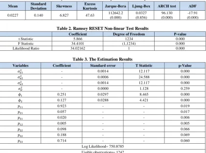
Table 3 shows the estimation results of the model (Markov-switching heteroscedasticity model).
Table 1. Summary Statistics (* Numbers in parentheses show p-values of tests.)
Mean Standard
Deviation Skewness
Excess
Kurtosis Jarque-Bera Ljung-Box ARCH test ADF
0.0227 0.140 6.827 47.63 112642.2
(0.000) 0.0327 (0.856) 96.130 (0.000) -17.91 (0.000)
Table 2. Ramsey RESET Non-linear Test Results
Coefficient Degree of Freedom P-value
t Statistic 5.866 1234 0.000
F Statistic 34.4101 (1,1234) 0.000
Likelihood Ratio 34.02162 1 0.000
Table 3. The Estimation Results
p-Value T Statistic Standard error Coefficient Variables 0.000 12.117 0.0014 0.000 24.588 0.0006 0.000 12.117 0.0014 0.259 1.128 0.0000 -0.000 8.465 0.0297 0.251 0.000 4.421 0.0288 0.127 0.019 -0.923 0.017 -0.057 0.006 -0.020 0.005 -0.005 0.066 -0.098 0.069 -0.188 0.060 -0.714
The variances of error terms of transitory component are statistically significant, and p-values of all three are less than 5%. However, the corresponding variance for the permanent component is statistically insignificant. Values of and are 0.25 and 0.12, respectively, and both have a p-value less than 5%, which shows that they are statistically significant. According to the magnitude of , about 40% of current values of the transitory component is explained by previous values (2 days ago). In addition, transition probabilities are all significant at 5% and 10%. The existence of high and medium variance states is very important for both investors and speculators in the stock market and higher levels of risk encourage them to demand higher returns. According to probability values, one can calculate the expected duration of every regime. The expected
duration for state 1 (low-variance) is
days,
the expected duration for state 2 (medium-variance) is
days, and for state 3 or high-variance
states, the corresponding value is
days. As
seen, the expected durations for different regimes are different. The duration for low-variance state is the longest, and the duration for high-variance state is short-lived and reverts to normal level quickly. To eliminate risks, risk averse investors should choose the buy-and-hold strategy instead of chasing-the-wind strategy.
For assessing the quality of regime classification in the Markov switching model, the regime classification
measure (RCM), proposed by Ang and Bekaert (2002) is calculated. For this 3-state model, the statistic is as follows:
∑ ∏ (10)
Where is the probability of being
in a certain regime at time t. In fact, this measure is a sample estimate of the variance of probability series. It stands on the idea that perfect classification of a regime would infer a value of 0 or 1 for probability series and be a Bernoulli random variable. This measure could have values between 0 and 100. A good regime classification has low RCM values. 0 value shows regime classification is perfect and 100 value indicates that regime classification is weak. As a result, a value of 50 can be used as a benchmark (Chan et al., 2011). In this paper, the RCM measure for the transitory component is 25.64, which shows the UC-MS model is able to distinguish quite confidently which regimes are occurring at each point in time.
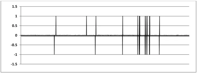
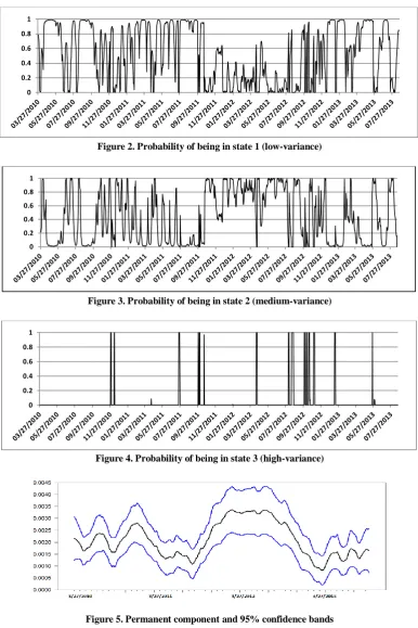
The following figures show actual data, the permanent component, and the probability of being in states 1, 2 and, 3.
Figure 1. Actual data
Figure 2. Probability of being in state 1 (low-variance)
Figure 3. Probability of being in state 2 (medium-variance)
Figure 4. Probability of being in state 3 (high-variance)
Figure 5. Permanent component and 95% confidence bands
0 0.2 0.4 0.6 0.8 1
0 0.2 0.4 0.6 0.8 1
5. Discussion and Conclusions
The unobserved component Markov-switching model helps to understand the source of mean reverting process and the resulting predictability. A random walk process usually describes the permanent component, and the transitory one is an autoregressive stationary process. Regarding real data, the stock return is a mixture of two processes. Thus, identifying the dominant component is important.
In this paper, the stochastic behavior of the Tehran Stock Exchange returns is examined using the Engel and Kim (1996) model. That is, stock returns are decomposed into permanent and transitory components using the unobserved component Markov-switching model. This approach allows analyzing the impact of shocks of permanent and transitory components like the study by Soleimani, Falahati, and Rostami (2016). In their study, using monthly Tehran stock market data, they decomposed stock returns using the state space model with Markov switching heteroscedasticity. However, the difference between this paper and their study is that they consider UC-MS model with two states of variances (high and low) in both permanent and transitory components.
The results show interesting conclusions. First, the results confirm the validity of using the UC-MS model in examining Tehran’s stock returns. Second, in the transitory component, about 40% of current values are defined by two previous periods (2 days ago), and it has a three-state Markov-switching heteroscedasticity, which was confirmed by under the value of RCM standing under 50. Third, the expected duration for the low-variance state, 13 days, is the longest, and the expected duration for the high-variance state, 4 days, is the shortest. Therefore, like previous studies such as Chen and Shen (2012) and Soleimani, Falahati, and Rostami (2016), results show that high-variance regimes are short-lived and go back to normal levels quickly. Fourth, the number of being in state 3 is high in year 2012. The main reason for that may be the presidential election in this year, which increases the uncertainty in the stock market, yet the permanent component in this period is relatively stable.
References
1) Albert, J. H. and Chib, S. (1993). Bayes Inference via Gibbs Sampling of Autoregressive Time Series Subject to Markov Mean and Variance Shifts.
Journal of Business and Economic Statistics, 11, 1-15.
2) Ang, A. and Bekaert, G. (2002). Regime Switches in Interest Rate. Journal of Business and Economic Statistics, 20, 163-182
3) Bhar, R. and Shigeyuki, H. (2004). Empirical Characteristic of Permanent and Transitory Components of Stock Returns: Analysis in a Markov-Switching Heteroscedasticity Framework. Economic Letters, 82, 157-165.
4) Camerer, C. (1989). Bubbles and Fads in Asset Prices. Journal of Economic Surveys, 3(1), 1-41. 5) Campbell, J. and Mankiw, G. (1987). Are Output
Fluctuation Transitory? Quarterly Journal of Economics, 102, 857-880.
6) Carter, C. K. and Kohn, R. (1994). On Gibbs Sampling for State Space Models. Biometrika, 81, 541-553.
7) Chan, K., Treepongkaruna, S., Brooks, R., and Gray, S. (2011). Asset Market Linkages: Evidence from Financial, Commodity and Real Estate Assets. Journal of Banking and Finance, 35 (6),1415-1426.
8) Chen, Sh. and Shen, Ch. (2012). Examining the Stochastic Behavior of REIT Returns: Evidence from the Regime Switching Approach. Journal Economic Modeling, Vol. 29, 291-298
9) Clark, P. (1987). The Cyclical Component of U.S. Economic Activity. Quarterly Journal of Economics, 102, 797-814.
10)Diebold, F. X., (1986). Modeling the Persistence of Conditional Variances: A Comment. Economietric Reviews, 5 (1), 51-56.
11)Engle, R. and Lee, G. (1992). A Permanent and Transitory Component of Stock Returns Volatility. University of California, San Diego Discussion paper. 92-44.
12)Engle, R. and Chowdhury, M. (1992). Implied ARCH Models from Option Prices. Journal of Econometrics, 52, 289-311.
13)Fama, E., French, K. (1988). Permanent and Transitory Component of Stock Prices. Journal of Political Economy, 96(2), 246-273.
14)Fama, E., Fischer, L., Jensen, M., and Roll, R. (1969). The Adjustment of Risk Prices to New Information. International Economic Review, 10. 15)Friedman, B. and Laibson, D. (1989). The
Movement in Stock Prices. Brooking papers of Economic Activity, 2, 137-189.
16)Gelfand, A. and Smith, A. (1990). Sampling-based Approaches to Calculating Marginal Densities. Journal of the American Statistical Association, 85, 398-409.
17)Hamilton, J. (1989). A New Approach to the Economic Analysis of Nonstationary Time Series and the Business Cycles. Econometrica, 57, 357-384.
18)Hamilton, J. and Susmel, R. (1994). Autoregressive Conditional Heteroscedasticity and Changes in Regime. Journal of Econometrics, 64, 307-333.
19)Hammoudeh, Sh. and Choi, K. (2007). Characteristic of Permanent and Transitory Returns in Oil-Sensitive Emerging Stock Market: The Case of GCC Countries. Journal of International Financial Market, Institutions and Money, 17, 231-245.
20)Kim, Ch. and Kim, M. (1996). Transient Fads and the Crash of ’87. Journal of Applied Econometrics, 11(1), 41-58.
21)Kim, Ch. and Nelson, Ch., Startz, R. (1991). Mean Reversion in Stock Prices? A Reappraisal of the Empirical Evidence. Review of Economic Studies, 58, 515-528.
22)Kim, Ch. and Nelson, Ch. (1998). Testing for Mean Reversion in Heteroskedastic Data II: Autoregression Tests Based on Gibbs Sampling-Augmented Randomization. Journal of Empirical Finance, 8(4), 385-396.
23)Kim, Ch., Nelson, Ch. and Startz, R. (1998). Testing for Mean Reversion in Heteroskedastic Data Based on Gibbs Sampling-Augmented Randomization. Journal of Empirical Finance, 5, 131-154.
24)Kim, Ch., Nelson, Ch. (1999). State Space Models with Regime Switching; Classical and Gibbs Sampling Approaches with Applications. The MIT Press, Cambridge, Massachusetts, London, England.
25)Le Roy, S. and Porter, R. (1981). The Present-Value Relation: Test Based on Implied Variance Bounds. Econometrica, 49(3), 555-574.
26)Najarzadeh, R., Sahabi, B., and Soleimani, S. (2013). The Relationship Between Inflation and Inflation Uncertainty in the Short and Long Run: State Space Model with Markov Switching
Heteroscedasticity. Journal of Economic Research, 18 (54), 1-25.
27)Nazifi Naeini, M. and Fatahi, Sh. (2012). Compering Regime Switching GARCH Models and GARCH Models in Developing Countries (case study of IRAN). Journal of Analisis Financiero, 60-68.
28)Poterba, J. and Summers, L. (1988). Mean Reversion in Stock Prices: Evidence and Implications. Journal of Financial Economics, 22, 27-59.
29)Schaller, H. and Van Norden, S. (2002). Fads or Bubbles? A Journal of The Institute Advanced Studies, Vienna, Austria, 27.
30)Schwert, W. (1990). Stock Volatility and the Crash of ’87. The Review of Financial Studies, 3, 77-102.
31)Shiller, R. (1981). Do Stock Prices Move too Much to Be Justified by Subsequent Changes in Dividends? The American Economic Review, 71(3), 421-436.
32)Shiller, R. (1984). Stock Prices and Social Dynamics. Brookings papers on Economic Activity, 457-498.
33)Soleimani, S., Falahati, A., and Rostami, A. R. (2016). Permanent and Transitory Components of Stock Returns: An Application of State Space with Markov Switching Heteroscedasticity. Journal of Economic Modeling Research, 7(25), 69-90. 34)Summers, L. (1986). Does the Stock Market
Rationally Reflect Fundamental Values? Journal of Finance XLI, 591-601.
35)Watson, M. (1986). Univariate Detrending Models with Stochastic Trends. Journal of Monetary Economics,18, 49-75.
36)West, K. (1988). Bubbles, Fads and Stock Prices Volatility Test: A Partial Evaluation. National Bureau of Economic Research, Working paper. 2574.
Not’s
i