THE DYNAMICS OF MANUFACTURING INDUSTRY AND THE RESPONSE TOWARD BUSINESS CYCLE

THE DYNAMICS OF MANUFACTURING INDUSTRY AND

THE RESPONSE TOWARD BUSINESS CYCLE

Yati Kurniati Yanfitri 1

The role of the manufacturing industry in the economy has expanded significantly from 19 percent

in 1990 to 26 percent in 2009, while its labor absorption only increased from 10 percent to 12.2 percent.

The cycle of the manufacturing industry has been in line with the economic growth. This study explores

the implications of the firm-level heterogeneity over the business cycle. By using the panel multinomial

logit, it shows that firms with less capital and small size have greater probability to exit the industry during

the boom/ bust period. Sensitivity of the company to changes in capital is greater during the boom period.

Only highly productive firms enter and begin production during recessions. Companies with higher

productivity rate also have greater probability to enter the market. In contrast, higher production cost and

higher market concentration increase the probability for smaller companies to exit from the industry.

1 Researcher of Econoomy in Bureau of Economy Research (Biro Riset Ekonomi/BRE), Directorate of Research in Economy and Monetery Policy (Direktorat Riset Ekonomi dan Kebijakan Moneter/DKM) of Bank of Indonesia. All opinions within this paper is the author»s personal view and do not reflect the official the policy of DKM or Bank of Indonesia. E-mail: [email protected], dan [email protected]

Abstract

JEL Classification JEL Classification JEL Classification JEL Classification

JEL Classification: D24, L6, E32

Keywords: Production, Cost, Capital and Total Factor Productivity, Industry Studies Manufacturing,

I. INTRODUCTION

For more than twenty years, the role of manufacturing industry in economy of Indonesia has substantially increased, from 19% to GDP in 1990 to 26% in 2009 (Figure II.1). Although during the years 1990-2008, the industrial sector also experienced a decline in growth due to economy crisis. But on the other hand, the employment in manufacturing rose slightly, only from 10% to 12%.

In general, the dynamics of industrial sector move in line with economic growth. When the Asian crisis hit Indonesia in 1997/1998, the GDP in 1998 grew negatively by 13.3% which was also followed by a decline in growth in the manufacturing sector amounted to 15.4% (Figure II.2). A sharp decline in manufacturing output in 1998 was also followed by a sharp decline in employment in the manufacturing sector that is equal to 9%.

Figure II.1

The Contribution of the Main Sectors Toward Economy

The significant contribution of manufacturing sector to the economy led makes the dynamics of the manufacturing sector inseparable factor in economic cycles. Boom and bust cycles in economy are often associated with a number of companies that enter and exit an industry. The enterprise»s dynamic also affects the decrease of output and employment opportunities in manufacturing sector.

The numbers of companies that come and go also influence the macroeconomic fluctuations for several reasons. First, these dynamics may occur due to the structure of the economy when facing shocks or policy changes. Second, the number of enterprises that enter and exit can be used to see the implications of a positive (boom) or negative (bust) shock.

Figure II.2

The Growth of GDP and Manufacturing Sector Year 1994-2009

% PDB

Manufacturing Industries (%) Agriculture (%)

Mining and Quarrying (%) Financial, Ownership and Business (%) 0

10 20 30 40 50 60 70

93 94 95 96 97 98 99 00 01 02 03 04 05 06 07 08 09

-Manufacturing GDP

1994 1997 2000 2003 2006 2009

25 -20 -15 -10 -5 0 5 10 15 20 25

Several studies provide empirical evidence of the influence of business cycles in the dynamics of the manufacturing industry. McQueen and Thorley (1993) stated that production capacity in the U.S. manufacturing industry will decline and slow down during the recession.

Most studies analyze the relationship between the characteristics of a manufacturing company with the economic cycle that focus on developed countries2_{. No studies that conduct} analysis to show a pattern for the manufacturing sector in business cycles, particularly in developing countries. Explicitly, this study aims to (i) find out the effect of differences in the boom/bust cycle of the level of enter/exit of companies, (ii) to investigate the characteristics of companies that in and out into the industry during the boom/bust period, and (iii) to measure the effect of the change of characteristics of the enterprises toward the opportunities for companies that enter and exit the industry during the period of boom/bust.

This study is composed in several sections. Section 2 describes the theoretical background and literature review. Section 3 discusses the methodology and data used. Section 4 presents a descriptive analysis of companies that enter and exit. Section 5 explains the data processing and Section 6 presents some conclusions.

II. THEORY

For company to exist, it will try to maximize profits. Therefore, the profit and growth opportunities factor for this sector will be a great attraction to enter a particular industry. On the other hand, other factors such as cost of production costs and other costs are also highly

considered by these companies to invest in the industry. In addition, the market characteristics, whether the industry is a perfectly competitive market, a monopolist, or between them, will affect the company»s level of economies of scale in producing goods which in turn also affect

the decision to enter/exit the industry.

Based on the theory of corporate behavior, the decision to enter the industry is based on the comparison between the additional benefits and costs. Starting from a profit maximization efforts π (Q) = TR(Q) - TC(Q), there are 3 conditions faced by the companies which namely (i) P = MR > AC (Stay or entry industry) where AC = AFC + AVC, (ii) P = MR = MC = AVC (Shutdown point), (iii) P = MR < AVC (Exit industry). These conditions are illustrated in Figure II.3.

Based on these equations, the company will maximize profits at P = MR = MC. At the point of M (zero profit) company will produce the goods at the level of MR=MC=AC. This means, in these conditions the company does not have a preference to remain or leave the

The amount of ATC (Average Total Cost) varies depending on the characteristics of the market. In a perfectly competitive market, there are no barriers to enter the market and no company has the power to control prices at a certain level. Industry, with a characteristic of a perfectly competitive market, will reach ATC at the lower output level compared to the imperfectly competitive market. Companies that produce goods under the ATC will grow their costs faster than their increases in output. While in imperfect competition market, the ATC curve is relatively flat, so that the zero-profit level (ATC=MC) can be achieved with a higher production output than a perfectly competitive market. The consequence of this characteristic is that small companies will find it difficult to enter the market.

In addition to the ATC, the barriers to entry factor also affect the company»s decision to enter or leave the industry. In a perfectly competitive market, this barrier does not exist, but to imperfect markets, constraints take place in the form of advertising, law, etc. These barriers lead to the increased costs to enter the market.

Based on this, it can be seen that the companies that survive in the market are the ones with an income at least equal to ATC, while the companies that can not generate revenue to cover the level of ATC will leave the industry.

company. While the point M» or called the ≈shutdown point∆, the company will suffer losses when producing output. At this level, or can be called also the level when the company take the decision to exit the industry, company revenue is only enough to cover variable costs and losses as much as the fixed costs. When the price determined by the company is under the AVC, the company will minimize losses by exiting the industry (Figure II.3).

Figure II.3

Behavior of the Company in Maximizing Profit

Price, AC, MC

MC

AC AVC

d

q M»

M d

Ps P

Zero - profit point

Shutdown point

0

(.)

≠

∂

∂

q

c

Based on the above explanation, the company will act rationally to produce at the level of the maximum profit. The function of a company can be written as follows. For each period t, company i is assumed to produce the optimum amount of goods q*_it with prices P_t in the following profit function:

where c_it (.) is the production cost incurred by the companies to manufacture goods as much as q*_it , X_it the vector representing the characteristics of the company, Z_t is other exogenous vectors that affect corporate profits.

The company will remain in production if the revenue gained is greater than or equal to production costs that should be deployed. Meanwhile, if the revenue is less than the cost of production, the company will stop producing.

If there is a company that requires an entry cost to operate, the company»s profit function becomes:

where η is the entry cost to start producing

The equation above is the equation at one point in time, while the equation for the multi-period can be written as follows:

If the current level of production period affects production costs in the next period

( ), then the decision to produce of a company is a dynamic equation

that can be written as follows:

A company would choose to produce in period t if the value of production is greater than the value of no production:

(II.2) (II.3) (II.4) (II.5)

)

|

,

(

)

,

(

X

Z

=

p

q

−

c

X

Z

q

π

0

)

,

(

0

)

,

(

0

1

<

≥







=

Z

X

Z

X

if

if

Y

π

π

)

1

(

)

|

,

(

)

,

(

~

−

−

−

=

t it

it

X

Z

p

q

c

X

Z

q

η

Y

π













=

Π

∑

it

X

Z

E

.

Y

]

~

[

)

,

(

δ

π

(

[

0

]

[

(

)

|

]

)

max

)

(

{q it it t it it

it

q

E

V

q

V

⋅

+

>

⋅

=

In the multi-period model, the entry cost to into the industry lays in the relationship between export activities in 2 consecutive years.

In addition to the theory of inter-temporal production, related with the level of entry/exit of companies from the industry, there are some new theories that support that concept. Joseph Schumpeter (1942) stated that the dynamics of the enterprise is a «creative destruction process which is later considered as the main cause of economic fluctuations. Schumpter stated production activities with the latest process and product innovation will be created continuously while the old process/items will be destroyed. This process serves to explain the growth and business cycles. Industry can have a different variation associated with the level of production units that utilize new technique or a level where the outdated production units are destroyed.

On the other hand, some scholars do not agree with the basic idea of creative destruction. Caballero and Hammour (1994) stated that the outdated production process is out of the industry due to a decline in demand, which in turn cause a reduction in production. Caballero and Hammour (2005) also questioned the view which states that the recession will increase the reallocation. They questioned the view that the company will replace any work that is removed during contraction by creating new jobs during the recovery period (panel (d) Diagram II.1). As depicted in panel (a) - (c) Diagram II.1, the restructuring of jobs during the recession may be positive, zero, or negative. This effect depends on the movement of economic contraction or recovery.

There are several studies that measure the factors that cause the level of entry and exit in the manufacturing sector. Shapiro (1997) found that the relationship between the level of entry and exit of the company is positively related to productivity. The entering or exiting process of a company is a part of the change process in which a large number of new companies replace a large number of the older ones. Therefore, the high entry rates of these companies are often associated with high rates of innovation and increased efficiency. The implications of the increase in manufacturing productivity are consistent with the highest level of entry/exit experienced by the manufacturing industry countries (Marcos and Jaumandreu, 2004).

Several other studies on the determinants of the entry and exit of a company within the industry were brought up by Audretsch (1995). Audrestch concluded that ratio entry/exit of a (II.6)

)

0

(

)

0

(

>

>

=

it

q

V

q

V

]

0

|

)

(

[

]

0

|

)

(

[

~

1 *

1

⋅

>

>

⋅

=

+

it

δ

E

V

q

δ

E

V

q

π

)

1

.(

]

0

|

)

(

[

]

0

|

)

(

[

*

− +

+

⋅

>

−

⋅

=

>

+

−

+

it

t

q

E

V

q

E

V

q

c

Y

company is closely linked to company size and age. On the other hand, Marcos and Jaumandreu (2004) showed the important role of competitive pressure (the increase of penetration in import markets which opened at extraordinary speed) and structural changes through a creative destruction process, which is by the displacement of inefficient enterprises.

One study that tried to explain the behavior of companies in developed countries conducted by Austin and Rosenbaum using the U.S. manufacturing industry data, to analyze the level of entry and exit based on a fairly large sample of 4-digit U.S. manufacturing industries. The market growth significantly improves (reduce) the level of entry (exit). Growth and profits (measured by using the price if industry-margin of the increasing entry rate) are also two factors that cause the companies to enter into the industry. Capital as a fixed cost measurement approach is also one barrier to exit the industry. In this study, Austin and Rosenbaum also add market concentration variables that also influence the level of entry and exit.

Another study conducted for the manufacturing industry in China (Yang, 2004) which analyzed the behavior of companies that survive, entered, and exited based on company size, labor productivity, and corporate efficiency index. The researcher concluded that a competitive selection process began to take shape in China, with the newly entering companies contribute substantially to the growth and productivity.

Diagram II.1.

Industrial Restructuring Process

(a) Restructuring Increases

(b) Restructuring is Unchanged creation destruction

creation destruction

(c) Restructuring Decreases

creation destruction

(d) Unemployment Recession

(II.9) Studies in developing countries conducted by the OECD (2001) presented a summary of empirical studies related to productivity and dynamics of company. Productivity can be measured by (1) Changes in productivity in each company (relative to the market) (2) reallocation process obtained from the process of expansion and contraction of existing enterprises, or from the entry/exit process of company to/from industry (the dynamics of the company). These studies divided the factors that influence the dynamics of the company into 4 major sections, which are company size, company age, productivity, technology and innovation, ownership structure, and other factors (minimum efficiency of scales, industrial concentration cycle factor). Most companies with large scale have a small tendency to leave the industry.

III. METHODOLOGY

III.1. Estimation Method for Logistic Panel

This research analyzes the opportunities for the company»s presence in an industry where every company has an opportunity to (i) enter the industry, (ii) remain in the industry, or (iii) exit the industry. Because of the nature of these endogenous variable categories, then multinomial logit model is used in this study.

The multinomial logit model is one of the choice model in which the individual (i) has the

choice of (j) at time (t), where the choices are more than 2 j=1,2,...j. Unlike probit, logit models are not limited to normally distributed data (Train, 2003). In general, the probability of individuals to take an option j is:

where,

This specification indicates that the utility U_ij is the maximum utility among all other options, for example when compared with the utility U_ik for j,k  K. In this case, V_ij shows that option j chosen by individual i from the total K options available.

In the above equation, the independent variables are divided into 2, which is constant

(w), and the independent variable that varies among options ( Z_ij ) By using equation (7) and the assumption of logit distribution, the probability of individual i to take the option j is:

V_ij = θT_x i j = β

T _Z i j + γ j

T_w

P_i (j) = P(U_{i j} = max U_{i k} ) = P(U_{i j} > U_ik for all k K)

= P(ε_{i k} = ε_{i j} ) < V_ij - V_ik)

In the multinomial logit, we need to identify the referred option. If option C is the choice of reference, then the probability of option A to be selected from C is:

where

The same goes for option B when relatively compared to the reference category C,

Where

Thus, for each option A, B and C, the probability of each to be selected corresponds to this equation:

To solve the multinomial logit equation , maximization of likelihood function is taken and shown in the following equation:

(II.11) (II.12) (II.16) (II.10)

∑

∑

=

=

=

e

e

e

e

j

Y

P

)

(

e

PC

PA

=

i

X

X

X

ZA

=

α

+

α

+

...

+

α

i ZB i i

e

PC

PB

=

i

X

X

X

ZB

=

β

+

β

+

...

+

β

(II.13) (II.14) (II.15) ZB ZA i

e

e

PC

+

+

=

1

1

e

e

e

PA

+

+

=

1

e

e

e

PB

+

+

=

1

i JA JB

i i n i JB i JA

i PB PA PB

PA

L − −

=

− −

=

∏

Based from the function L, the interpretation of changes of probability of A is formed on the change of independent variables, which are as follows:

Based on these equations there are 2 factors that cause changes in the probability of choosing A; which are the changes in the independent variable X that is own effects and cross effects. The probability calculation above represents the entire estimated observation period. In the data panel, the opportunity to choose option j based on the characteristic X_it, has the variation between individuals and over time, so that the individual utilities to take the option j in time t for individual n is:

where ε_njt has a variation between individuals, time, and alternatives. Specifications of maximized logit function for the panel equation is as follows:

By integrating the left hand side (LHS) and right-hand side (RHS), then the maximization is now done based on an integral function of L. In general case, the maximization of a function is performed by a small pace of change, h, for the whole interval function. This approach is known as the composite quadrature, which assumes that for the entire interval, the function is smooth and does not have a large variation (equally spaced points). A better approach for the maximization of the above integral function L is the adaptive quadrature that approaches the integral numbers with a particular value using a method to create the posterior distribution from the unobserved heterogeneity (Haan and Uhlendorff, 2006). Technically, this makes the step of this adaptive quadrature approach smaller than h for the intervals where these functions have greater fluctuations (heterogeneous).

(II.17) (II.18)

(

)

x

U

=

β

+

ε

da a f a X a X L ijt d N i T t J j j k k k it j j it ) ( ) exp( ) exp(

1 1 1

It is analogous to the specifications of the probability of each event to be selected, as shown in the previous equation, but this time, the probability for any individual (cross-section) can be obtained. Technically, the logistic panel estimation is done with STATA software3_{. Related} to the selection of fixed and random effects models, within STATA itself, there is no command for multinomial logit with fixed effect as there is no sufficient statistical evidence that the fixed effect can be adjusted by maximum likelihood. Estimation of the fixed effect model will generate an inconsistent and biased estimator (Bernard and Jensen, 2004). Thus, this study utilizes multinomial logit random effects.

III.2. Data, Conceptualization and Measurement of Data Variable

Referring to the theory and previous empirical studies, the empirical model estimated in this paper is given below. The plus and minus signs on each variable representing the initial hypothesis proposed, and applied to both the boom and bust period

3 STATA belongs to and is copyrighted by Stata Corp LP.

Y = AKα_L1-α

ln Y= ln A + αlnK + (1 - α) lnL

P(Entry) = f (size+_{, cr} -- _{, capital} +_,TFP+_{, labor cost of production )}

P(Exit) = f (size--_{, cr} -- _{, capital ,TFP , labor cost of production} +₎

The data used is data from Survey of Medium and Large Industrial year 1990-2007. The level of entry/exit/remaining of the companies computed using the following definition: - Companies that enter the industry are categorized as a company that exist in period t, but

non-exist in the period t-1.

- Companies that exit or leave the industry are categorized as a non-exist in period t, but exist in period t-1.

- Companies that survive/remain in the industry are companies that exist in at the very least 3 consecutive periods of period t-1, t and t +1.

The explanatory variables, used in the empirical model and the selection, are as follows: 1. Total Factor Productivity (TFP) = Calculation of TFP using Solow residuals and Cobb Douglas

functions. Cobb Douglas function can be written as follows:

sections methodology. Value of α and β will vary between sub-industry, depending on the characteristics of the industry, whether they have a production function of increasing returns to scale, decreasing returns to scale, or constant returns to scale. Calculation of technology by using the Solow residual does not take into account the impact of technology improvement caused by other sectors

2. Concentration Ratio (CR) = the level of market concentration to identify whether a particular industry is a group with a perfect competition market or monopoly. Concentration ratio value ranges from 0 to 1, where 0 indicates the characteristics of perfect competition, while 1 indicates monopolistic market. The CR is calculated using the following equation:

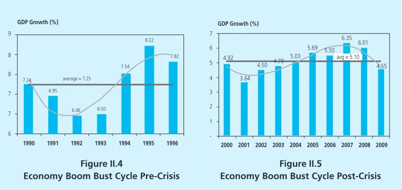
Figure II.4

Economy Boom Bust Cycle Pre-Crisis

Figure II.5

Economy Boom Bust Cycle Post-Crisis 3. Dummy variable (boom/bust) shows the business cycle of the economy4_{. This dummy is}

calculated based on the deviation of economic growth for a specified period against the

average over time. Boom period is the period when economic growth is above the average, and the opposite is the bust period.

The average that is used as a basis to determine the period of boom/bust, are divided into 2 parts: pre-crisis period (1990-1996) with an average economic growth of 7.25% per year, and the period after the crisis (2000 -2006) with an average growth of 5.10% per year (Figure II.4 and II.5).

4 The boom bust cycle can also be calculated using the real wage variable (appendix), and the periodization of boom bust, without any significant difference compared to the calcualation using PDB. Thus, this study remain using the GNP to define boom bust period.

9

8

8

7

7

6

GDP Growth (%)

7.24 6.95

6.46 6.50 7.54

8.22

7.82

1990 1991 1992 1993 1994 1995 1996 average = 7.25

7

6

5

4

3

2

1

-2000 2001 2002 2003 2004 2005 2006 2007 2008 2009 GDP Growth (%)

4.92

3.64 4.50 4.70

5.03 5.69 _5.50

6.35 6.01

4.55 avg = 5.10

CR = 10 top output

Based on the mean and deviation calculation, the following result shows up: - Boom Period took place in 1990, 1994, 1995, 1996, 2005, and 2006

- Bust period took place in 1991, 1992, 1993, 1997, 1998, 1999, 2000, 2001-2004 4. Other variables used are the amount of production labor that shows the size of the company,

the company»s capital and wage of production labor

IV. RESULT AND ANALYSIS

IV.1. The Growth Of Industrial Sector

The industrial sector represents a significant contribution to the sector in the economy. Within the year of 1967-1997, growth in industrial sector was almost always higher than the economic growth. Economic growth during this period had the average of 6.1% while the growth in industrial sector reached 10.3% per year. During this period various policies were undertaken to improve the growth of industrial sectors such as import substitution and export orientation (Figure II.6).

Figure II.6

The Growth of Industrial Sector Year 1967-2009

Major changes occurred in the year 1997-2004, during the period of economy crisis where industrial sector grew only by 3.1%. After 1997, the growth in industrial sector has always been under the economic growth. As a result of decreased growth, the government put more efforts to revitalize and restructure the industry. Based on the contribution of industrial sector to the economy of Indonesia until 2004, in average, industrial sector is accounted for 26.9% of the economy, which cover the 86.5% contribution of the non-oil industries.

Source : Ministry of Industry

Industry Growth GDP Growth (%)

25

20

15

10

5

0

-5

-10

-15

-20

In detail, the sub-industry of transportation, machinery, and equipment have an increasing role. In 1999, sub industry contributed only 5.9% for the economy, while in 2000 increased to 20.7% and the increase is consistent until 2004 which reached 26.5%.

After the industrial revitalization was applied in 2004, All sub-industries grew in positive manner. In Table 1 it can be seen that the industry of food, wood and forest products experienced positive growth. The biggest growth is experienced by the sub-industry of transportation, machinery, and equipment (12:46%). On the other hand sub-industry will also have a major contribution to the economy that will reach 28.95% in 2009. However, the employment in this sector is relatively small. The highest level of employment is shown by the sub-industry of food, beverages, and tobacco.

The capacity utilization rate also varies sub-industry during 2004-2009. The largest capacity utilization is owned by the sub paper and printing industry, while the industry that is experiencing

Table II.1

Contribution of Sub-Industry/Industry toward Economy

Growth (%)

1 Food, Beverages, and Tobacco Products 1.39 2.75 7.22 5.05 2.34 3.66 2 Textiles, Wearing Apparel; Dressing of Leather 4.06 1.31 1.23 -3.68 -3.64 -5.15

3 Wood and Products of Wood -2.07 -0.92 -0.66 -1.74 3.45 2.44

4 Paper and its Products; Publishing, Printing 7.61 2.39 2.09 5.79 -1.48 0.61 5 Coke, Refined Petroleum Products, Chemicals;

Rubber and Plastics Products 9.01 8.77 4.48 5.69 4.46 3.50

6 Cement and Other Non-Metallic Mineral Products 9.53 3.81 0.53 3.40 -1.49 -1.50 7 Basic Metals, Fabricated Metal Products -2.61 -3.70 4.73 1.69 -2.05 0.55 8 Machinery, Transport, and Equipment 17.67 12.38 7.55 9.73 9.79 8.75

9 Others 12.77 2.61 3.62 -2.82 -0.96 2.82

Total 7.51 5.86 5.27 5.15 4.05 3.97

1 Food, Beverages, and Tobacco Products 28.10 28.18 27.95 29.79 30.40 30.91 2 Textiles, Wearing Apparel; Dressing of Leather 13.80 12.20 11.91 10.56 9.21 8.75

3 Wood and Products of Wood 5.60 5.55 5.82 6.19 6.43 6.64

4 Paper and its Products; Publishing, Printing 5.30 5.41 5.24 5.12 4.56 4.51 5 Coke, Refined Petroleum Products, Chemicals;

Rubber and Plastics Products 16.90 12.26 12.56 12.49 13.53 13.52 6 Cement and Other Non-Metallic Mineral Products 4.20 3.89 3.80 3.70 3.53 3.48 7 Basic Metals, Fabricated Metal Products 2.90 2.88 2.69 2.58 2.57 2.45 8 Machinery, Transport, and Equipment 22.50 28.72 29.09 28.70 28.97 28.95

9 Others 0.80 0.92 0.94 0.85 0.80 0.78

Total 100.00 100.00 100.00 100.00 100.00 100.00

No

2004 2005 2006 2007 2008 2009*

Manufacturer of

Share in the Industry (%)

2004 2005 2006 2007 2008 2009*

high growth in capacity utilization is the shipping industry due to the empowerment of domestic industry and government regulations that encourage this sub-industry to do more export.

On the contrary a decline in capacity utilization is shown by the industry of fertilizers, chemicals, and rubber goods, especially in the year 2008. This is the result from a lack of supply of natural gas which serves as raw materials and energy.

In terms of export, the industries of Palm/Palm Oil processing, Iron Steel, Machinery and Automotive, Textile, Rubber Processing Industry, and Electronics are the largest contributors to the non-oil exports. Generally, the non-oil manufacturing industries, during the first four years, have a tendency of increased export value, except in 2009 due to declining demand from abroad due to the global crisis.

Table II.2

Average Sub-Industry Growth in 2004-2009

1. Food, Beverages, and Tobacco Products 4.59 514,557 2. Textiles, Leather, and Footwear 6.65 485,955

3. Wood and Product Wood 4.91 133,119

4. Paper and Printing 7.82 42,595

5. Fertilizer, Chemicals, and Rubber Goods 10.63 143,273 6. Cement and Non-Metallic Mineral Products 10.13 5,918 7. Basic Metals, Iron and Steel 3.94 341,388 8. Machinery, Transport, and Equipment 12.46 96,510

9. Others 10.2 887,853

Total Total Total Total

Total 8.568.568.568.568.56 2,635,6902,635,6902,635,6902,635,6902,635,690

Industry (in ISIC 2 digit)

Growth (%)

Number of Cummulative Labor in 5 years (people)

Table II.3

Sub-Industry Contribution to the Economy in 2004-2009

Percent (%)

Food, Beverages, and Tobacco Products 28.1 28.18 27.95 29.79 30.40 30.91

Textiles, Leather, and Footwear 3.8 12.20 11.91 10.56 9.21 8.75

Wood and Product Wood 5.6 5.55 5.82 6.19 6.43 6.64

Paper and Printing 5.3 5.41 5.24 5.12 4.56 4.51

Fertilizer, Chemicals, and Rubber Goods 16.9 12.26 12.56 12.49 13.53 13.52 Cement and Non-Metallic Mineral Products 4.2 3.80 3.80 3.70 3.53 3.48

Basic Metals, Iron and Steel 2.9 2.88 2.69 2.58 2.57 2.45

Machinery, Transportation, and Equipment 22.5 28.72 29.09 28.70 28.97 28.95

Others 0.8 0.92 0.94 0.94 0.80 0.78

Total Industry Total Industry Total Industry Total Industry

Total Industry 100.00100.00100.00100.00100.00 100.00100.00100.00100.00100.00 100.00100.00100.00100.00100.00 100.00100.00100.00100.00100.00 100.00100.00100.00100.00100.00 100.00100.00100.00100.00100.00

2004 2005 2006 2007 2008 2009*

Table II.4

The Capacity Utilization Rate of Sub-Industries in 2004-2009

1 Steel Industry 53.1 56.3 57.8 60.5 59.8 56.62

2 Non-Metall Industry 63.62 65.68 62.8 65.1 63.6 54.89

3 Downstream Metal Industries 56.05 59.9 62.7 61.1 61.9 60.74

4 Industrial Machinery 63.4 67.1 67.7 69.7 71.3 66.76

5 Textile Industry 67.7 69.4 70 75.81 68.2 70.52

6 Various Industries 58.5 59.6 58.75 58.97 58.53 59.41

7 Shipping Industry 50 50 60 70 80 50.00

8 Two-wheeled Motor Vehicle Industry 79.4 78.4 67.5 71.5 73.8 74.27 9 Fou-wheeled Motor Vehicle Industry 43.8 59.1 32.9 45.7 57.04 47.69

10 Electronics Industry 67 68.3 70 70 73 68.21

11 Telematics Industry 65 65 68.1 68.2 68.4 65.88

12 Food, Beverage and Tobacco Industries 55.2 56.1 55.8 57.6 58.32* 55.69 13 Industrial Products and Forest Products 64.8 64.7 63.4 63.5 62.98* 64.42

14 Paper and Printing Industry 79.6 83.2 88.5 88.8 92.37* 84.06

15 Fertilizer, Chemical and Rubber Products Industry 71.1 72.3 67.1 67.2 65.56* 71.07 16 Cement & Non-MetaIlic Minerals Industry 61.1 62.5 64.4 71.7 75.40* 61.60

Average Industry 63.1 65.1 63.8 66.9 67.93* 64.20

No Group 2004 2005 2006 2007 2008 2009*

Table II.5

Export of Manufacturing Sub-Industries in 2004-2009

1 Processing Oil/Palm Oil 4,840.30 5,419.19 6,407.27 10,476.83 16,168.07 13,249.46 2 Iron Steel, Machineries and Automotive 4,581.84 5,949.69 7,712.68 9,606.92 11,814.98 10,720.08

3 Textiles 7,626.15 8,584.85 9,422.75 9,790.09 10,116.35 9,947.69

4 Rubber Processing 2,954.10 3,545.82 5,465.16 6,179.87 7,579.66 6,947.25 5 Electronics 7,142.50 7,853.03 7,200.19 6,359.73 6,806.70 6,656.97 6 Processing of Copper, Tin, etc 2,165.08 3,133.52 4,133.97 6,156.04 5,660.67 5,713.40 7 Pulp and paper 2,817.61 3,257.48 3,983.27 4,440.09 5,219.62 4,859.62 8 Wood Processing 4,461.62 4,476.25 4,757.59 4,485.14 4,206.12 4,372.99 9 Basic Chemistry 2,640.07 2,750.22 3,521.44 4,492.50 3,738.35 4,019.17 10 Food and Beverage 1,440.12 1,647.92 1,866.00 2,374.83 3,104.85 2,736.36 11 Power Tools 1,232.73 1,456.03 1,770.93 2,148.88 2,390.24 2,259.58 12 Leather, Leather Goods, and Shoes/Footwear 1,553.04 1,683.69 1,913.17 2,006.60 2,260.46 2,148.35

Total of 12 Large Industry 43,455.17 49,757.71 58,154.42 68,517.92 79,066.08 73,702.89 Total Industry 48,660.11 55,566.99 64,990.33 76,429.60 88,351.70 82,314.00 Non Oil and Gas 55,939.28 66,428.36 79,589.15 92,012.32 107,894.15 100,163.05

Oil and Gas 15,645.33 19,231.60 21,209.48 22,088.57 29,126.27 25,970.29

No Description 2004 2005 2006 2007 2008 2009*

IV.2. The Model Estimation Result: Panel Multinomial Logit

The growth of industrial sector experienced downward trend over the last few years. Before the crisis, the manufacturing sector grew by an average of 11.8%5_{(yoy), whereas after} the crisis the growth fell to 4.6%6 _{(yoy). This decline may be the correspond to output the} growth due to the increased exit rate post-crisis or the entry of companies with lower output, while the companies that took the leave are the company with high output.

5 The average of growth of industry 1994-1996 6 The average of growth of industry 2000-2009

Table II.6

The Import of Manufacturing Sub-industries 2004-2009

1 Iron Steel, Machineries and Automotive 13,620.20 17,531.04 17,031.41 20,539.04 39,978.13 33,689.13 2 Electronics 2,048.47 2,413.48 2,488.31 4,035.98 13,444.71 10,445.41 3 Basic Chemistry 5,690.64 5,935.32 6,315.39 7,115.75 10,716.70 9,641.02

4 Textiles 1,036.36 1,026.87 1,085.68 1,192.00 3,901.78 3,023.93

5 Food and Beverage 1,390.67 1,914.52 2,178.23 3,616.14 3,157.97 3,440.27 6 Pulp and Paper 1,299.76 1,298.95 1,392.04 1,692.60 2,518.49 2,279.81

7 Power Tools 724.42 877.79 852.98 1,118.31 2,470.79 2,036.17

8 Fertilizer 431.99 518.87 624.65 761.78 2,337.64 1,843.82

9 Others Chemical Goods 1,078.06 1,167.23 1,170.03 1,293.82 1,845.64 1,671.44

Total of 9 Large Industry 27,320.57 32,684.07 33,138.71 41,365.42 80,372.42 68,071 Total Industry 31,550.79 37,300.34 38,624.63 48,084.08 91,800.67 7,816,689 Non Oil and Gas 34,792.48 40,243.21 42,102.59 52,540.61 98,644.41 84,372.53

Oil and Gas 11,732.05 17,457.68 18,962.87 21,932.82 30,552.90 28,142.35

No Description 2004 2005 2006 2007 2008 2009*

Table II.7 The Rate of Companies that Enter, Exit or Remain in the Manufacturing Industries (%)

Year Stay Entry Exit

1991 75.9 17.1 7.0

1992 78.3 15.2 6.5

1993 82.6 11.1 6.3

1994 83.1 11.7 5.2

1995 75.8 17.4 6.8

1996 51.9 14.9 33.2

1997 81.0 8.0 11.0

1998 84.5 8.4 7.1

1999 87.6 7.8 4.6

2000 77.5 5.7 16.9

2001 80.1 15.1 4.8

2002 87.3 4.7 8.0

2003 73.6 5.1 21.2

2004 73.0 9.5 17.5

2005 71.7 7.8 20.5

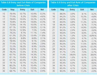
The number of firms that enter, exit, or remain in the industry generally does not change from year to year. On average, companies that survive in an industry are 76.8% per year, while the entrance is 11.2% per year. The amount is almost similar to the level of the company that took an exit which is by 12%.

In 1996 and 1997 a significant increase in exit rate occurred which reached 33.2% and 11.2%. It shows that in times of crisis or bust of the economy, there were more companies that left the industry while the number of companies that joined declined.

When decoded into 2-digit SITC code, before the crisis, half of the sub-industries had the tendency of a balance number of entering and exiting company. In this period, the sub-industry of refined petroleum based articles (23) and basic metal products (27) had the highest average entering company, around 10-11% per year.

On the contrary happens after the crisis, almost the entire sub industries had more companies that took an exit. Even some of the sub industries had an increased net exit rate. For example, the textile sub-industry, before the crisis, had 0.2% companies that left, while after crisis, it increased to 4.5% per year. Similar pattern are shown in the apparel and food industry.

Table II.8 Entry and Exit Rate of Companies before Crisis

Code Stay Entry Exit Net

15 78.4% 10.7% 10.9% -0.3%

16 77.0% 9.2% 13.8% -4.6%

17 79.8% 10.0% 10.2% -0.2%

18 70.8% 14.4% 14.8% -0.3%

19 75.9% 14.1% 10.0% 4.1%

20 67.1% 13.9% 19.0% -5.1%

21 79.5% 12.9% 7.5% 5.4%

22 79.2% 9.7% 11.1% -1.4%

23 61.3% 25.2% 13.4% 11.8%

24 82.4% 8.8% 8.8% 0.1%

25 78.9% 12.0% 9.1% 2.9%

26 77.4% 12.7% 9.9% 2.9%

27 72.2% 18.2% 8.9% 10.0%

28 78.9% 12.0% 9.1% 3.0%

29 78.2% 13.3% 8.5% 4.7%

30 65.7% 20.0% 14.3% 5.7%

31 81.1% 10.6% 8.3% 2.3%

32 67.7% 20.4% 11.9% 8.5%

33 79.1% 10.7% 10.2% 0.5%

34 80.2% 9.3% 10.4% -1.1%

35 75.4% 11.1% 13.5% -2.4%

36 68.7% 15.2% 16.1% -0.9%

Table II.9 Entry and Exit Rate of Companies after Crisis

Code Stay Entry Exit Net

On the other hand, there are several companies that have more companies joining per year post-crisis, such as the sub-industries of office equipment, accounting and computers (30) and motorcycles and bicycles production (34). This is in line with the movement of transportation sub-industry that contributes the most to the total industrial output.

The processing of multinomial logit panel is applied to the overall sub-industries (ISIC 2 digits). Based on this result, we obtain the factors that affect the entry/exit rate during the boom/bust in the economy. These factors were divided into 3 parts: company characteristics (size, capital costs, productivity), market characteristics and macroeconomic conditions (boom/ bust of economy).

IV.2.1. Company»s Capital

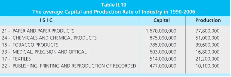
Company»s capital is the component of the value of buildings, lands, vehicles, and equipments. The greater the company»s capital is, then the greater the chance of entering the industry. Capital is the company»s fixed costs. To make a profit, the company will produce in large capacity.

Table II.10

The average Capital and Production Rate of Industry in 1990-2006

I S I C Capital Production

21 - PAPER AND PAPER PRODUCTS 1,670,000,000 77,800,000 24 - CHEMICALS AND CHEMICAL PRODUCTS 875,000,000 51,000,000

16 - TOBACCO PRODUCTS 785,000,000 39,600,000

33 - MEDICAL, PRECISION AND OPTICAL 603,000,000 16,800,000

17 - TEXTILES 514,000,000 21,200,000

22 - PUBLISHING, PRINTING AND REPRODUCTION OF RECORDED 477,000,000 10,100,000

When we observe the relation between sensitivity of capital of each sub-industry to the probability of a company to enter during the boom, most of the sub-industry has a positive relationship to capital. The highest sensitivity is shown by the non-metal products (26) sub-industry. On the other hand, sub-industries with large capital also have a positive sensitivity to changes in capital. It gives the reasons why during the boom period there was an increase of production value of manufacturing companies.

The opposite occurred during the bust, the amount of capital of the companies does not significantly affect the chances of entering the industry. Even in some industries there are negative tendencies to enter the industry. The biggest negative sensitivity is possessed by the paper and paper products (21) industry. A negative coefficient is also shown during the bust; the companies that entered the industry have a relatively smaller capital than companies that survive. These empirical results also showed little growth during the bust caused by the industrial sector. Companies have no incentive to enter the industry and/or the companies that entered the industry have a small amount capital and thus the level of production is also small.

Behavior of the companies that exit from the market showed very little difference during the boom and bust. The estimation result shows that the behavior is consistent with the initial hypothesis, where the increase in the capital will reduce the chances of the company to enter the industry.

In we view in more detail of the behavior of companies during the bust, the sensitivity of capital growth to the probability of the companies to exit the industry showed a negative relationship. The role of capital to significantly influence the companies to exit can be seen in the tobacco sub-industry (16). The industries with large capital category also have a great sensitivity to changes in capital. During the bust, capital changes do not affect the company»s decision to exit or remain in the industry.

The estimation results also showed that during the boom, 1% addition of the company»s capital will increase the chances of companies to survive in the industry, with the same magnitude. During the boom, the furniture industry (36) has the great sensitivity to changes in capital. In addition, other industries also have greater sensitivity to changes in capital.

The estimation results show that the policies which have implications in increasing the

company»s capital will be effective during the boom and bust of economy, but the impact will be greater during the boom. This will improve the number of entering companies and reduce the number of exiting companies, especially the policies of capital increase in sub-industries

IV.2.2. Size of company

In general, the entering companies are relatively small in size, except for companies at the health equipment sub-industry. The same way, the exiting companies are usually comparably small, except in the sub-industry of machine, radio, and telecommunications. In total, during the boom period, the reduction of the total size of the company is influence by the entering and exiting dynamics of the companies. If the sizes of the company are compared during the period of boom and bust, there will be no significant difference in the both time.

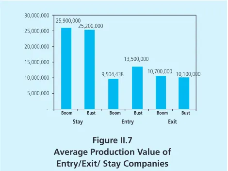
Similarly from the point of view of production value, the company that entered the industry has smaller production, except for the base metal, telecommunications and medical equipment sub-industry. And the companies that exit also have smaller production, except for the base metals sub-industry. During the boom in the economy, the value of production of the remaining companies is greater than during the bust, but the dynamics of companies that enter and exit cause a decrease to the total production value.

Figure II.7

Average Production Value of Entry/Exit/ Stay Companies 30,000,000

25,000,000

20,000,000

15,000,000

10,000,000

5,000,000

-25,900,000 25,200,000

9,504,438 13,500,000

10,700,000 10,100,000

Boom Bust Boom Bust Boom Bust

Stay Entry Exit

In the results using the multinomial logit panel, these are also indicated by the negative

coefficient on the bust and boom. This difference also shows that companies that enter and exit during the bust and boom in the economy have a relatively smaller size than the previously remaining companies. These empirical results also show that during the boom even though the

number of companies that enter into the industry is larger, but the size is comparably smaller than during the bust.

of production labor is an obstacle for the company to profit. In contrast to the boom period where the growth and profit are expected and this will benefit even the companies with small number of worker.

If we view the sensitivity of each industry during the boom and bust, all industry behaviors in total also appear in most of sub-industry. During the bust, printing sub-industry (22) enters the industry with the least work force. Meanwhile, during the boom, the companies under the textile sub-industry (17) are smaller in size.

What is interesting that the results obtained from the estimated multinomial logit panel is that in some sub-industry the effect of the rising number of production workers increases the chances of companies to enter the industry. During the boom, such sub-industries are like the tobacco (16), radio and telecommunications (32) and rubber and plastics (25) industries. While during the bust, the enlargement of company size in tobacco sub-industry (16) will increase the chances of companies to enter into the industry. This is consistent with the descriptive analysis presented earlier, in the recent times of boom; the sub-industry that absorbs the most man power is the radio industry and telecommunications.

The size of companies that leave the industry is also relatively smaller than the average company to survive. In addition, the companies that exit during the boom, are relatively smaller than the bust. This is indicated by the negative sign/direction coefficients.

On the other hand, the negative coefficient indicates that a greater amount of production labor will lower the probability of the exiting companies, or in other words, companies will choose to survive in the industry. Sensitivity is greater in the boom than during the bust period. During the boom, the bigger the size of the company will reduce the probability of company to exit larger than during the bust. Or in other words, companies are more easily to exit during the bust.

If we view in more detail the sensitivity of company size toward probability of companies to exit the industry, almost all companies have the same behavior with the total industry. During the

bust, the largest sensitivity of the size of companies in related to the probability of companies to exit the industry, lies within the tobacco sub-industry (16). Meanwhile, during the boom, the largest sensitivity of company size on the probability for companies to exit the industry lies in the

furniture sub-industry (36).

IV.2.3. Production Cost

The greater the production cost which was approached by the workers» wages will reduce the opportunities for companies to enter the industry. Such behavior may appear during the boom or bust in the economy. During the economic bust, sensitivity on the increase of production cost is smaller than in the period of boom. Negative sensitivity also shows that entering companies have lower production cost than companies that remain in the industry. On the other hand, the panel multinomial logit empirical results also show that the cost of production of a company that enters the industry during the boom period is smaller than during the bust.

These behaviors that arise in the entire industry are also happening in most of sub-industry. During the bust in the economy, a raise in production costs will cause the biggest impact on food and beverage industry (15), while during the boom, he garment industry (19) has the greatest sensitivity to the cost of production.

On the other hand, probability for companies to exit the industry is affected by the positive relationship between the production cost and labor cost. The higher the labor costs will increase the chances of the company to exit during the economic bust. Meanwhile, during the boom, production cost does not affect the company»s decision to quit the industry.

During an economic bust, a highest positive sensitivity of production cost on the probability of companies to exit the industry, lies in the tobacco industry (16), while during the boom lies in the chemical and chemical products industry (24).

The policy implication of this analysis is to reduce the cost of production especially during

the bust in the economy, because it will affect the company»s decision to enter or exit the industry. While the reduction of production costs during the boom, will only reduce the number companies that enter the industry.

IV.2.4. Technology of the Company

During the boom periods, the companies enter the industry with a higher level of technology. In total, during the boom, the technology that enters the industry becomes smaller. For the most company, during the boom and bust there is no significant difference in technology.

Most of the manufacturing sub-industries have a greater dependence toward labor and the opposite toward capital. The addition of 1 unit of capital good gives a smaller increase than the addition of 1 unit of labor.

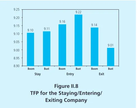
Figure II.8

TFP for the Staying/Entering/ Exiting Company

large dependence on labor force with an average coefficient of 0.17. Meanwhile the machine, telecommunications, computers sub-industries have a greater dependence on capital goods (0.22).

The total capital and labor coefficients also showed the trend that manufacturing industries have a pattern of increasing returns to scale, except for processed oil sub-industry. The biggest largest output driven by the increase of input is shown by the sub-industries of radio, television, and telecommunications and a few industries that tend to have the high levels of technology.

Therefore, the increase in the number of workers in technology-based industries is required, and with the combination of high level of labor and capital, it will produce more output.

In addition to the role of capital and labor, technology also has a contribution to the output. The one with the largest technology are the sub-industries of rice processing, products of oil and gas, and communication equipment. While the sub-industries of tobacco, clay, and photography equipment have a relatively smaller technology.

Compared to the year 1990, the level of technology owned by the industry is currently increasing. However, during 2000-2006 the technological growth decelerated. The largest improvement of technology was experienced by sub-industry of artificial fibers (average growth7 of 14.85% per year), while the smallest growth in technology was in the electronic components (average growth of 2.50% per year).

In the both period (boom/bust), the company that enters the industry has a greater level of technology compared to the company that survives/exit of the industry. Company technology

7 The average growth of technology in 2000-2006

9.25

9.20

9.15

9.10

9.05

9.00

8.95

8.90

9.10 9.11

9.16 9.22

9.14

9.01

Boom Bust Boom Bust Boom Bust

shows the utilization of technology in producing output, so that the higher the technology, the more output the company will produce. Logit panel estimation results show that in the bust period, the company that enters the industry has the technology that is smaller than during the boom. The estimation results are consistent with initial hypothesis.

When viewed in detail, during the bust the company that enters with the lowest technology is the timber and wooden products industry (20). Meanwhile, during the economic boom, companies that enter the industry have the greater technology. The greater the company»s technology will increase the probability of companies to enter the industry even greater. The largest sensitivity is presents in the food and beverage industry (15). The higher the technology is, the bigger probability for the company to enter the industry.

While the exiting companies have a tendency to have higher level of technology compared to their own industry (both in the boom and bust). During the bust, the technology of the exiting company is more sophisticated than the boom. When viewed in more detail, the metal sub-industry (28) has the probability to exit the industry with the largest increase in technology, while during the boom the furniture industry (36) has the highest probability.

The calculation result of logit panel multinomial shows that during the economic bust, an increase of 1% in technology will decrease the probability for companies to enter and increase the probability for companies to exit. So at the bust, in total, the companies that survive are relatively small and at the boom period, an increase of 1% of technology will lead higher probability for companies to enter than to exit.

IV.2.5. Characteristics of Market

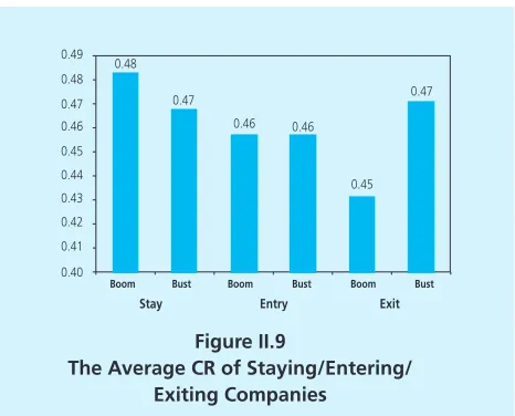
The level of market concentration which shows the degree of economies of scale also varies in each industry. Sub-industry with a large concentration has monopolistic characteristics, so that the cost to enter the industry is relatively large. The companies that have large market concentration include the industries of tobacco, plastics, metals, office machinery, radio and communications and medical equipment. These sub-industries, in general, have an entry rate below the industry average.

The opposite occurs on the characteristics of companies that exit the industry. The companies exit the industry that led to the monopoly more easily, especially during the bust of economy. Meanwhile, during the boom, the market characteristics are not a factor affecting the company»s decision to remain or exit the industry.

V. CONCLUSION AND RECOMMENDED POLICIES

Based on the results of qualitative and quantitative analysis which has been conducted, several things can be concluded as follows:

1. Changes in economic conditions is indicated by the difference in the level of companies enter/exit the industry. During the economic crisis in 1997-1998, there was a high exit rate, while entering companies were relatively fewer.

2. Characteristics of the companies that enter into the industry:

- In the boom period, the probability for the company to enter the industry is in line with the accretion of capital and technology, and is negatively related to the amount of labor, production costs, and the level of market concentration.

- The probability of companies to enter the industry during the bust period will be augmented with the decrease in capital and size, labor costs, technology and market concentration

3. There are some industries that require large size both in terms of capital and labor to enter the industry, such as sub-radio and telecommunications and rubber and plastic industries. 4. Characteristics of companies that exit the industry:

Figure II.9

The Average CR of Staying/Entering/ Exiting Companies

0.48

0.47

0.46 0.46

0.45 0.47 0.49

0.48

0.47 0.46

0.45

0.44

0.43

0.42

0.41

0.40

Boom Bust Boom Bust Boom Bust

- In periods of boom/bust, the probability of companies to exit the industry will be greater if the labor cost of production increases, if the size of the company is reduced, and if there is a decline in capital

Based on these conclusions we can be draw several policy recommendations. Sensitivity of the companies towards the capital is larger during the boom than bust. It gives the consequence; policies to increase the capital would be more effective in improving the probabilities for companies to enter the industry during the boom. While increasing the company»s capital during the bust will prevent the companies to exit the industry. Therefore, in order to strengthen the manufacturing industry during the bust, greater incentives are needed to improve the company»s capital.

The results of the data also show that large sized companies has a great chance to survive in the industry, related to the economic of scale, while small companies are more prone to enter and exit during the boom/bust. During the bust of economy, labor costs of production need to be suppressed because it will affect the company»s decision to enter or exit the industry. While the reduction of production costs during the boom, will only reduce the number of company that enters the industry.

Ahn, Sanghoon, (2001). "Firm Dynamics and Productivity Growth : A Review of Micro Evidence From OECD Countries", OECD Economics Department, Working Paper No. 97.

Austin, John S and David I. Rosenbaum. " The Determinants of Entry and Exit Rates Into US Manufacturing Industries", Review of Industrial Organization, Vol.5 No. 2.

Bernard, Andrew B. and J.B. Jensen. (2004). "Why Some Firms Export," The Review of Economics and Statistics, Vol. 86, No. 2.

Caballero, R. J. and M. L. Hammour, (1994). "The Cleansing Effect of Recessions," American Economic Review, No.84, 1350-1368.

Caballero, R. J. and M. L. Hammour, (2005). "The Cost of Recessions Revisited: A Reverse-Liquidationist View," American Economic Review, No.84, 1350-1368.

Davis, S.J. and J.C. Haltawanger, (1990)."Gross Job Creation and Destruction: Microeconomic Evidence and Macroeconomic Implications," NBER Macroeconomic Annual V, 123-168. Holzl Werner and Leopold Sogner, (2004). "Entry and Exit Dynamics in The Austrian

Manufacturing Industries." Vienna University of Economics and Business Administration, Working Paper No. 36.

Ilmakunnas, Pekka and Jukka Topi (1999). "Microeconomic and Macroeconomic Influences on Entry

and Exit of Firms." Review of Industrial Organization No. 15, 283-301.

Lee, Y. and T. Mukoyama, (2008). "Entry, Exit and Plant-Level Dynamics over the Business Cycle," Federal Reserve Bank of Cleveland Working Paper 07-18R.

Martin-Marcos, Ana and Jordi Jaumandreu, (2004). "Entry, Exit, and Productivity Growth: Spanish

Manufacturing during The Eighties." Spanish Economic Review No. 6, 211-226.

McQueen, Grant and Thorley, Steven, (1993). "Asymmetric business cycle turning points." Journal of Monetary Economics, 31, 341-362.

Yang, Qing Gong, (2004). "Entry, Exit and The Dynamics of Productivity Growth in Chinese Manufacturing Industry", ESRC Centre for Business Research, University of Cambridge, Working Paper No. 284.

APPENDIX

Marjinal Effect √ Entry Bust

ISIC Size Capital Wage Market Concentration Technology Constant

15 16 17 18 19 20 21 22 23 24 25 26 27 28 29 31 32 33 34 35 36 Total NS 0.052 *** NS NS (0.035) *** (0.030) *** (0.074) *** (0.114) *** NS (0.102) *** (0.030) *** (0.030) *** (0.034) *** (0.001) *** (0.077) *** 0.007 *** (0.000) * NS (0.056) ** NS (0.022) *** (0.014) *** (0.002) *** (0.003) ** NS NS (0.002) ** NS (0.006) *** NS NS NS (0.003) *** NS 0.003 ** NS NS NS (0.000) *** NS NS (0.001) ** NS (0.002) *** (0.036) *** (0.060) *** (0.025) *** (0.002) *** 0.030 *** (0.023) *** 0.044 *** NS NS 0.028 ** 0.025 *** (0.015) *** NS 0.000 *** 0.041 ** (0.008) *** 0.000 *** NS 0.026 * NS NS (0.020) *** (0.048) *** (0.163) *** 0.105 *** (0.017) *** (0.070) ** (0.159) *** NS 0.276 *** NS 0.214 *** (0.268) *** (0.120) *** NS (0.003) *** 0.412 *** 0.010 *** (0.000) *** (0.065) * NS (0.176) *** (0.058) *** (0.011) *** (0.027) *** 0.006 ** (0.027) *** 0.002 ** (0.075) *** (0.109) *** (0.124) *** (0.073) *** NS (0.096) *** (0.071) *** NS (0.021) *** (0.000) *** (0.094) *** 0.008) *** NS (0.004) *** (0.069) *** (0.010) *** NS (0.022) ** 0.199 *** 0.090 *** 0.104 *** (0.070) *** 0.142 *** 0.583 *** 0.260 *** 0.508 *** NS 0.418 *** 0.179 *** (0.049) *** 0.029 ** (0.003) *** 0.203 *** 0.071 *** (0.000) *** (0.052) *** 0.139 ** (0.049) *** (0.058) *** (0.005) ***

Marjinal Effect √ Exit Bust

ISIC Size Capital Wage Market Concentration Technology Constant

ISIC Size Capital Wage Market Concentration Technology Constant 15 16 17 18 19 20 21 22 23 24 25 26 27 28 29 31 32 33 34 35 36 Total (0.063) *** 0.000 *** (0.107) *** (0.020) * NS (0.014) *** (0.104) ** (0.021) ** NS (0.016) ** 0.019 *** (0.092) *** (0.050) * (0.023) ** NS NS 0.192 *** NS NS (0.004) *** 0.000 *** (0.077) *** NS 0.000 * 0.009 *** 0.004 *** NS NS NS NS 0.000 ** 0.004 *** 0.001 *** 0.010 *** NS 0.003 *** 0.007 *** 0.001 * 0.008 ** 0.000 * NS NS 0.002 *** 0.006 ***

(0.081) *** (0.055) ** 0.104 *** (0.227) ***

(0.000) ** NS 0.000 *** 0.000 **

(0.081) *** (0.052) 0.086 *** NS

(0.073) *** (0.100) *** 0.083 *** (0.192) **

(0.088) *** NS 0.088 *** NS

(0.015) *** (0.040) *** 0.022 *** (0.084) ***

NS (2.526) *** NS (1.083) ***

(0.019) *** NS 0.024 *** (0.090) *

NS NS 0.000 * (0.004) *

(0.042) *** NS 0.014 *** 0.210 ***

(0.031) *** NS 0.024 *** NS

(0.037) *** (0.201) *** 0.038 *** NS

NS NS NS 0.337 **

(0.047) *** NS 0.027 *** 0.194 ***

(0.052) *** NS 0.023 *** NS

(0.023) *** 0.063 *** NS 0.173 ***

(0.063) *** (0.526) *** 0.049 *** NS

NS NS NS (0.018) **

(0.053) * 0.349 *** 0.036 *** NS

NS NS 0.002 *** (0.029) ***

(0.006) *** (0.063) ** 0.014 *** NS

(0.078) *** (0.027) *** 0.074 *** 0.118 ***

Marjinal Effect √ Entry Boom

ISIC Size Capital Wage Market Concentration Technology Constant

15 16 17 18 19 20 21 22 23 24 25 26 27 28 29 31 32 33 34 35 36 Total (0.007)*** (0.000)*** (0.011)*** (0.002)*** (0.011)*** (0.018)** (0.001)*** (0.004)*** (0.001)* (0.005)*** (0.002)** (0.009)*** (0.000)*** (0.000)*** (0.003)*** (0.000)*** NS NS (0.007)** (0.011)*** (0.135)*** (0.008)*** (0.000)*** NS (0.001)*** (0.000)*** (0.001)** (0.002)*** (0.000)** (0.000)*** NS (0.001)* (0.000)*** NS NS (0.000)* NS (0.000)* (0.001)* NS (0.001)* NS (0.010)*** (0.000)*** 0.006*** (0.009)*** 0.007* NS 0.055*** NS 0.023*** (0.009)* NS NS (0.002)** (0.002)* NS NS NS NS (0.077)*** NS (0.011) (0.039)** NS NS 0.001*** (0.000)*** 0.004*** 0.001*** 0.005*** 0.020*** 0.001*** 0.001*** NS 0.002*** (0.001)*** 0.001*** 0.000** (0.000)*** 0.001*** 0.000*** NS NS (0.000)** 0.002*** 0.068*** 0.001*** (0.003)* (0.001)*** NS (0.006)*** NS (0.108)** 0.007** (0.015)*** NS NS (0.006)** (0.008)* (0.000)* (0.002)** (0.016)* (0.000)*** (1.000)* (0.001)*** NS (0.038)** 0.550*** (0.018)*** NS NS 0.000** 0.001* NS NS NS NS NS 0.002*** NS 0.001* NS NS NS 0.000** NS NS NS NS (0.061)*** NS

8 The branch of non oil and gas industry : industry of food, beverage, tobacco, transportation, machinery and equipment, fertilizer, chemical product, rubber product, textile, leather articles and footwear.

Code ISIC Description

15 16 17 18 19 20 21 22 23 24 25 26 27 28 29 30 31 32 33 34 35 36

The Code of Industrial Groups8

MANUFACTURE OF FOOD PRODUCTS AND BEVERAGES MANUFACTURE OF TOBACCO PRODUCTS

MANUFACTURE OF TEXTILES

MANUFACTURE OF WEARING APPAREL; DRESSING AND DYEING TANNING AND DRESSING OF LEATHER; MANUFACTURE OF MANUFACTURE OF WOOD AND OF PRODUCTS OF WOOD AND MANUFACTURE OF PAPER AND PAPER PRODUCTS

PUBLISHING, PRINTING AND REPRODUCTION OF RECORDED MANUFACTURE OF COKE, REFINED PETROLEUM PRODUCTS MANUFACTURE OF CHEMICALS AND CHEMICAL PRODUCTS MANUFACTURE OF RUBBER AND PLASTICS PRODUCTS MANUFACTURE OF OTHER NON-METALLIC MINERAL PRODUCTS MANUFACTURE OF BASIC METALS

MANUFACTURE OF FABRICATED METAL PRODUCTS MANUFACTURE OF MACHINERY AND EQUIPMENT N.E.C. MANUFACTURE OF OFFICE, ACCOUNTING AND COMPUTING MANUFACTURE OF ELECTRICAL MACHINERY AND APPARATUS MANUFACTURE OF RADIO, TELEVISION AND COMMUNICATION MANUFACTURE OF MEDICAL, PRECISION AND OPTICAL MANUFACTURE OF MOTOR VEHICLES, TRAILERS MANUFACTURE OF OTHER TRANSPORT EQUIPMENT MANUFACTURE OF FURNITURE; MANUFACTURE N.E.C.

Figure 1

Periodization of Boom Bust (Real Wages) Before Crisis

Periodization Boom/Bust of Economy (Real Wages)

-10 -5 0 5 10 15 20 25 30

1990 1991 1992 1993 1994 1995 1996 Real Wage

Figure 2

Periodization of Boom Bust (Real Wages) After Crisis

Real Wage Average Poly. (Real Wage ) 0

20 40 60 80 100 120 140 160 180

2000 2001 2002 2003 2004 2005 2006 2007 Real Wage

ISIC Coef L Coef K

15 16 17 18 19 20 21 22 23 24 25 26 27 28 29 30 31 32 34 35 36 37

Solow Residual Signification Test

Table 1.

Signification Test of Solow Residual

0.91** 0.22***

1.19 0.18***

1.12*** 0.16***

0.99 0.15

0.96*** 0.16***

1.06** 0.13***

1.18 0.14***

1.09** 0.16***

0.81 0.14***

1.14** 0.16***

0.96** 0.15***

1.13*** 0.17***

0.98 0.22***

1.02 0.19***

1.03 0.24***

0.81 0.27***

0.96 0.24***

1.14*** 0.27***

1.14*** 0.2***

1.05 0.24***

0.89*** 0.13***

0.86*** 0.2

Heustman Test Panel Solow Residual

Ho : difference in coefficients not systematic (fixed effect) Hi : difference in coefficients systematic (random effect) chi2(2) = (b-B)»[(V_b-V_B)^(-1)](b-B)

= 90.9 Prob>chi2 = 0.0000

ISIC Small Medium Big 15

16 17 18 19 20 21 22 23 24 25 26 27 28 29 30 31 32 33 34 35 36 37 Total

0% 100% 0% 2% 0% 66% 0% 0% 0% 0% 0% 49% 0% 0% 0% 0% 0% 0% 53% 0% 1% 0% 9% 14%

81% 0% 100% 98% 100% 34% 100% 70% 0% 0% 29% 38% 0% 0% 42% 0% 24% 0% 36% 28% 41% 100% 91% 63%

Distribution of Companies Based on Technologies Applied

Table 2. Distribution of Companies (2006) Based on Technologies Applied