Gabriel Caloz & Monique Dauge, Editors
DOMAIN DECOMPOSITION BASED NEWTON METHODS FOR
FLUID-STRUCTURE INTERACTION PROBLEMS
Miguel ´
Angel Fern´
andez
1, Jean-Fr´
ed´
eric Gerbeau
1, Antoine Gloria
2,3and
Marina Vidrascu
4Abstract. We review various fluid-structure algorithms based on domain decomposition techniques and we propose a new one. The standard methods used in fluid-structure interaction problems are generally “nonlinear on subdomains”. We propose a scheme based on the principle “linearize first, then decompose”. In other words we extend to fluid-structure problems domain decomposition techniques classically used in nonlinear elasticity.
R´esum´e. Nous faisons une revue de divers algorithmes de couplage fluide-structure bas´es sur des tech-niques de d´ecomposition de domaine et nous en proposons une nouvelle. Les m´ethodes classiquement utilis´ees en interaction fluide-structure sont g´en´eralement “non lin´eaires par sous-domaine”. Le sch´ema que nous proposons est au contraire bas´e sur le principe “lin´eariser puis d´ecomposer”. Autrement dit, nous ´etendons aux probl`emes d’interaction fluide-structure des techniques de d´ecomposition de domaine classiquement utilis´ees en ´elasticit´e non lin´eaire.
Introduction
In this paper we review various numerical methods to treat the interaction between an incompressible fluid and an elastic structure, and we propose a new approach based on a Newton algorithm and domain decompo-sition methods. To model the structure, we use 3D-shell elements, which allows us to use three dimensional consititutive laws (see [4–6]). Up to our knowledge, this is the first time such elements are used in fluid-structure interaction.
Fluid-structure algorithms are too numerous to be reviewed exhaustively. A classification of the various approaches is not obvious either. To begin with, we can consider two groups of methods: the “strongly coupled” and the “loosely coupled” schemes. This distinction is quite clear since it corresponds to a precise property: those schemes which can ensure a well-balanced energy transfer between the fluid and the structure can be called “strongly coupled”, the other ones are “loosely coupled”. All the methods presented in this study are strongly coupled. Loosely coupled schemes, which are very powerful in many applications but can be unstable in others, are not considered here. We refer for example to [12, 30] for explicit coupling schemes and to [15, 16] for a semi-implicit coupling scheme.
We can then distinguish “monolithic” and “partitioned” schemes. For example, an ad hoc solver whose purpose is to solve simultaneously the fluid and the structure typically leads to a monolithic scheme (see for
1
Project-team REO, INRIA Paris-Rocquencourt, 78153 Le Chesnay Cedex, France 2
CERMICS, Ecole Nationale des Ponts et Chauss´ees, 77455 Marne-la-Vall´ee, France 3
Project-teams REO & MICMAC, INRIA Paris-Rocquencourt, 78153 Le Chesnay Cedex, France 4
Project-team MACS, INRIA Paris-Rocquencourt, 78153 Le Chesnay Cedex, France
c
EDP Sciences, SMAI 2007
example [1, 10, 22, 23, 31, 32, 35]). On the other hand, coupling one fluid solver and one structure solver as black boxes clearly yields a partitioned scheme. Such a partitioned scheme can be strongly coupled as soon as sub-iterations are performed at each time step. The number of subsub-iterations being very large in some application, acceleration techniques have been investigated in several articles: for example Le Tallec and Mouro [25] propose a steepest descent approach, Mok, Wall and Ramm [28] propose an Aitken acceleration which is based on the two previously computed solutions, and Vierendeels [34] a least-square method which uses several previously computed solutions.
It is well-known, in particular since the work by Le Tallec and Mouro [25] and more recently by Depariset al.[8, 9], that structure problems can be tackled with domain decomposition approaches. Indeed, a fluid-structure problem can be viewed as a general continuum mechanics problem set on one domain which is split into a fluid part and a structure part. The fluid-structure coupling conditions then appear as the transmission conditions which ensure that the solution of the global problem is obtained by “sticking” the two sub-problem solutions. This point of view has been adopted in various studies, either with the so-called “Dirichlet-Neumann” algorithms (see for example [13, 21, 26]) or with “Neumann-Neumann” algorithms ( [8, 9]).
All these methods have been devised following the rule “apply domain decomposition to the nonlinear global problem and then solve on each subdomain the nonlinear problems”. On the contrary, in other fields – for example nonlinear elasticity [24] – domain decomposition is usually applied with the rule “linearize first, then solve the tangent problem using domain decomposition”. The purpose of this paper is to propose a fluid-structure algorithm based on the last rule. The resulting algorithm can be viewed as a monolithic scheme in the sense that we apply a Newton algorithm to the global fluid-structure problem. But it is more conform to the practical implementation to consider it as a partitioned scheme since the fluid and the structure are solved with two different solvers, with their own schemes, and can be run in parallel. Contrarily to the methods following the first rule, these solvers are only used to solve the tangent problems and to evaluate nonlinear residuals. The use of two different solvers has well-known advantages (re-usability of existing codes, flexible choice of the numerical methods adapted to each sub-problem,etc.). Compared to monolithic schemes presented in the literature [22, 23, 31], our approach may have another advantage: the use of domain decomposition methods to solve the tangent problem is expected to be more efficient than direct methods or iterative methods based on block-preconditioners.
In Section 1 we review some standard approaches to solve fluid-structure interaction problems, in particular those based on domain decomposition arguments, that use the so-called Steklov-Poincar´e operators. In Section 2 we recall the fluid and solid models and we set the main notations. The time scheme is presented in Section 3. In Section 4 the new algorithm is introduced. It is difficult to anticipate the advantages in terms of efficiency of the proposed approach. Nevertheless we propose in Section 4.2 a simplified complexity analysis whose conclusion may be sum up as follows: the more expensive the structure problem and nonlinear the fluid (let think of the Navier-Stokes equations but also of complex models for the fluid), the more competitive is expected this new formulation. Preliminary numerical results are reported on in Section 5. More extensive simulations and comparisons with existing methods will be proposed in a forthcoming work [14].
1.
Classical solution methods
In this section we briefly review the existing algorithms for the numerical solution of the nonlinear system arising in the time discretization of the fluid-structure problem with an implicit coupling scheme. These methods are typically based on the application of a particular nonlinear iterative method to three different formulations of the nonlinear coupled system.
such that
Formulation (I):
F(xf,γ) = 0,
S(xs,γ) = 0,
I(xf,xs) = 0.
(1)
Equations of (1)1 and (1)2 ensure the equilibrium of momentum when the fluid and the solid are subjected to
an interface displacement γ, whereas the last equation enforces the equilibrium of mechanical stresses at the interface.
Problem (1) can be reformulated in terms of γ by eliminating the fluid and solid unknowns xf,xs. This
yields to the so-called Steklov-Poincar´e formulation: Find the interface displacement γsuch that,
Formulation (II): Sf(γ) +Ss(γ) = 0. (2)
Here,Sf andSsstand for the fluid and solid Steklov-Poincar´e operators which can be defined as follows: for a
given interface displacementγ,Sf(γ) gives the stress exerted by the fluid on the interface, and analogously for
Ss. All these notations will be made precise below. In section 3.2, we shall describe the link between (1) and
(2).
Finally, the composition of the inverse operatorS−1
s with (2) gives rise to the so-called Dirichlet-to-Neumann
formulation:
Formulation (III): Ss−1 −Sf(γ)
−γ= 0. (3)
Formally speaking, Formulations (II) and (III) are similar. Nevertheless, we prefer to distinguish them since they correspond to different approaches in the literature. The denominations “Dirichlet-Neumann formulation” and “Steklov-Poincar´e formulation” are purely conventional (both of them clearly involve Steklov-Poincar´e operators).
The three following paragraphs address a brief state-of-the-art on the iterative methods for the numerical solution of (1), (2) and (3).
1.1.
Monolithic formulation
A common approach in the numerical solution of nonlinear systems, arising in implicit coupling, consists in applying a Newton based algorithm to the global formulation (1). This requires the repeated solution of a tangent (or approximated tangent) problem with the following block structure:
DxfF(xf,γ) 0 DγF(xf,γ)
0 DxsS(xs,γ) DγS(xs,γ)
DxfI(xf,xs) DxsI(xf,xs) 0
δxf
δxs
δγ =−
F(xf,γ)
S(xs,γ)
I(xf,xs)
. (4)
Newton algorithms based on the numerical solution of (4) in amonolithic fashion, i.e. using global direct or iterative methods, have been reported in [1, 10, 22, 32, 35]. It is worth noticing that such a monolithic approach makes difficult the use of separate solvers for the fluid and structure sub-problems. Alternatively, system (4) can be solved in apartitioned manner through a block-Gauss elimination ofδxf, which leads to the so called
block-Newton methods [17, 18].
1.2.
Dirichlet to Neumann formulations
Formulation (III) reduces problem (1) to the determination of a fixed point of the Dirichlet-to-Neumann operatorγ7→S−1
s −Sf(γ). This motivates the use of fixed-point based methods [25, 27–29]:
γk+1=ωkS−s1 −Sf(γk)
+ (1−ωk)γk, (5)
withωk a given relaxation parameter which is chosen in order to enhance convergence [7, 27, 28]. Alternatively,
solution of a tangent problem of the type
(J(γk)−I)δγ=− S−1
s −Sf(γk)−γk, (6)
where J(γ) stands for the Jacobian, or approximated Jacobian [21], of the composed operator γ 7→ S−1
s −
Sf(γ). It is worth noticing that exact Jacobian computations require shape derivative calculus for the fluid [19].
Let us also stress the fact that these methods are naturally partitioned.
1.3.
Symmetric Steklov-Poincar´
e formulation
The Dirichlet-Neumann formulations share a common feature: their implementation is purely sequential. The Steklov-Poincar´e formulation (2) may allow to set up parallel algorithms to solve the interface equation.
Following the presentation of Deparis et al.[8], the nonlinear problem (2) can be solved through nonlinear Richardson iterations:
P(γk+1−γk) =ωk(−Sf(γk)−Ss(γk)), (7)
for an appropriate choice of the preconditionerP, namely
Pk−1=αkSf′(γk)
−1
+ (1−αk)Ss′(γk)
−1
, (8)
where λ 7→ S′
f(β)·λ is the differential of Sf at β, and
Sf′(β)
−1
its inverse. This choice generalizes the standard preconditioners of linear domain decomposition methods (for which S′ =S). If α
k is 0,1 or 0.5 we
retrieve respectively Dirichlet-Neumann, Neumann-Dirichlet or Neumann-Neumann preconditioners. On the other hand, since equation (2) is nonlinear, one can apply a Newton method,
Sf′(γk) +Ss′(γk)(γk+1−γk) =−Sf(γk)−Ss(γk). (9)
which corresponds to the nonlinear Richardson iteration (7) preconditioned with Pk =Sf′(γk) +Ss′(γk). This
linear equation can be solved, for example, by a GMRES algorithm, with or without preconditioning. For instance, in [8] the authors propose to use the preconditioners (8).
The Newton method applied to the Dirichlet-Neumann formulation is not equivalent to the Newton method applied to the Steklov formulation, since the roles played by the fluid and by the structure are not symmetric in the first approach whereas they are in the second. After linearization, one cannot compose (6) withSs to
retrieve (9). Finally (8) is not equivalent to (9) since in general (A+B)−1=6 A−1+B−1.
The advantage of formulation (II) compared to formulation (III) is that the fluid and the structure sub-problems can be solved simultaneously and independently for the residual computation (right-hand sides of (7)) and the application of the preconditioner (S′f andSs′) as soon asα /∈ {0,1}. However, as we shall see in section
4.2, a simplified complexity analysis shows that the overall computational costs of both methods might be of the same order, for instance, whenever the cost of the fluid sub-problems solution is cheaper.
The formulations recalled in Sections 1.2 and 1.3 are first based on the coupling conditions, giving rise to a nonlinear equation on the interface, which involves nonlinear sub-problems. The algorithm we introduce in Section 4 first treats the nonlinearity of the whole problem through a Newton method, and uses a Steklov-Poincar´e formulation on the tangent problems.
2.
Mechanical setting
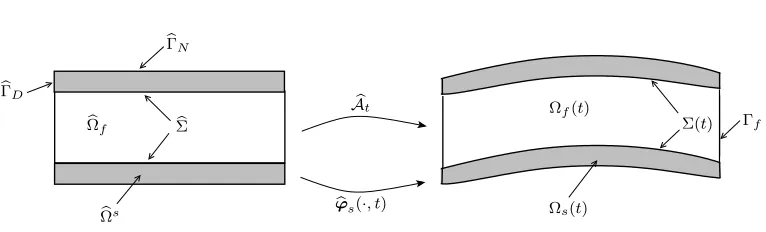
LetΩ =b Ωbf∪Ωbs be a reference configuration of the system, see Figure 1. We introduce the motion of the
solid medium
b
ϕs:Ωbs×R+−→R3.
The current configuration of the structure is then denoted by Ωs(t) =ϕs(Ωbs, t). We introduce the deformation
gradient Fbs(x, tb ) def
= ∇xbϕ
s(x, tb ), and its determinant Jbs(x, tb ) def
domain is given bydbs(bx, t) def
= ϕbs(bx, t)−xb. The fluid domain Ωf(t) is parametrized by the Arbitrary Lagrangian
Eulerian ALE mapping (see [11], for instance),
b
A:Ωbf×R+−→R3,
such that Ωf(t) =Ab(Ωbf, t). In the sequel we will use the notation Abt def
= Ab(·, t) and the superscriptb will be related to fields defined on the reference configurationΩbf orΩbs. In addition, for a given Eulerian fluid quantity
q(i.e. defined in Ωf(t) fort >0) we will denote its ALE description by bq, as a field defined inΩbf×R+as
b
q(x, tb ) =q Abt(x), t
, ∀x∈Ωbf. (10)
We introduce the deformation gradient of the fluid domainFbf(x, tb ) def
= ∇xbAb(x, tb ),and its determinantJbf(bx, t)def=
detFbf(bx, t). The displacement of the fluid domain is given bybdf(bx, t) def
= Ab(x, tb )−xb and its velocity by
b w def= ∂Ab
∂t.
b
Σ
b
Ωf
Ωf(t)
Σ(t)
Ωs(t)
b
At
b
Ωs ϕbs(·, t)
b
ΓN
b
ΓD
Γf
Figure 1. Parametrization of the domains Ωf(t) and Ωs(t).
The fluid-structure interface, namely∂Ωf(t)∩∂Ωs(t) is denoted by Σ(t), and Γf =∂Ωf(t)\Σ(t) stands for
the portion of the fluid boundary that is not shared with the boundary of the structure. The surface Γf is
assumed to be independent oft. The boundary ∂Ωbs of the reference configuration for the structure is divided
into three disjoint parts bΓD, ΓbN and Σ, with Σ(b t) = Abt(Σ). We denote byb n the outward unit normal on
the fluid boundary in the current configuration, and bynbs the outward unit normal on the reference structure
boundary.
2.1.
The coupled problem
We consider a Newtonian viscous, incompressible fluid with densityρf and dynamic viscosityµ. Its state is
described by its Eulerian velocityuand pressurep. The constitutive law for the Cauchy stress tensor is given by the following expression:
σ(u, p) =−pI+ 2µǫ(u),
with ǫ(u) =∇u+ (∇u)T/2. In absence of body forces, these unknowns satisfy the incompressible
Navier-Stokes equations in an ALE formulation:
ρf
∂u ∂t
b
x+ρf(u−w)·
∇u−div 2µǫ(u)+∇p= 0, in Ωf(t),
divu= 0, in Ωf(t),
σ(u, p)·n=g, on Γf,
where ∂ ∂t
b
x stands for the ALE time derivative,w
def
= wb ◦Ab−t1, andga given density of surface force.
The structure is supposed to be hyperelastic under large displacements and deformations. Its density is denoted by ρs. Its state is described by its displacement dbs and its first Piola-Kirchoff stress tensorTb. The
latter is related todbs as the gradient of an internal stored energy functionW(Fbs). The choice of the internal
stored energy will depend on the problem under consideration and will not change the setting of the fluid-structure problem. Assuming that the fluid-structure is clamped on ΓDand under no body and surface forces, these
unknowns are driven by the following elastodynamic equations
b Jsρs∂
2bd s
∂t2 −divxbTb=0, in Ωbs,
b
d=0, on bΓD,
b
T·nbs= 0, on bΓN.
(12)
The coupling between the solid and the fluid, namely equations (11) and (12), is realized through standard boundary conditions at the fluid-structure interface Σ(t) that ensure the balance of the mechanical energy over the whole domain. This is achieved by imposing three interface conditions:
• A geometrical condition enforcing the matching betweenϕsandAbon the interface
b
df =bds, on Σb. (13)
InsideΩbf, the fluid domain displacementdbf can be defined as an arbitraryL2-extension ofdbsover the
domainΩbf, namely,
b
df = Ext(bds|Σb) (14)
(see Remark 1 below).
• A kinematic condition enforcing the continuity of the velocities at the interface
u=∂dbs ∂t ◦Ab
−1
t , on Σ(t). (15)
• And a kinetic condition imposing the stress continuity at the interface
b
Tnbs=Jbfσ\(u, p)Fb
−T
f nbs, on Σb. (16)
To summarize, the fluid-structure system involving an incompressible viscous fluid and a hyperelastic structure is described in terms of the unknowns (u, p,bdf,dbs) satisfying the coupled problem (11)-(16).
Remark 1. In practice, we can choose as operator Ext a harmonic extension operator, by solving a Laplace
equation
−κ∆dbf = 0, on Ωbf,
b
df =bds, on Σb,
b
df =0, on Γbf,
(17)
whereκ >0is a given “diffusion” coefficient, that might depend ondbs. Other alternative extension approaches
can be found, for instance, in [2, 33].
Remark 3. For simplicity, we have only prescribed Neumann boundary conditions in (11). In practice we may use Dirichlet conditions on some part of the boundary.
2.2.
Weak formulation
Problem (11)-(16) can be reformulated in a weak variational form using appropriate test functions, performing integrations by parts and taking into account the boundary and interface conditions.
In what follows, we will make explicit the dependence of Ωf(t) and Σ(t) ondbf by introducing the notations
Ωf(dbf) def
= Ωf(t), Σ(bdf) def
= Σ(t).
Let (vcf,qb) ∈ [H1(Ωbf)]3×L2(Ωbf), multiplying the fluid problem (11) by (vf, q) = (vcf ◦ Ab−t1,qb◦Ab
−1 t )
integrating over Ωf(dbf) and after integrations by parts we get
d dt
Z
Ωf(dcf)
ρfu·vfdx+
Z
Ωf(dcf)
divhρfu⊗
u−w dcfi·vfdx+
Z
Ωf(dcf)
σ(u, p) :∇vfdx
− Z
Σ(dcf)
σ(u, p)·vf·nda−
Z
Γin−out
g·vfda−
Z
Ωf(dcf)
qdivudx= 0,
where
w dcf
=∂dcf ∂t ◦Ab
−1 t .
For the structure, multiplying (12) bycvs∈[HΓ1D(Ωbs)]
3, integrating overΩb
sand integrating by parts, one gets
Z
b Ωs
ρ0∂ 2dc
s
∂t2 ·cvsdˆx+
Z
b Ωs
∂W
∂F (I +∇cds) :∇cvsdˆx− Z
b Σ
∂W
∂F (I +∇dcs)nbs·vcsdˆa= 0,
whereρ0=Jbsρs. Therefore, taking into account the coupling condition (16), it follows that
d dt
Z
Ωf(dcf)
ρfu·vfdx+
Z
Ωf(dcf)
divhρfu⊗
u−w dcf
i
·vfdx+
Z
Ωf(dcf)
σ(u, p) :∇vfdx
− Z
Γin−out
g·vfda−
Z
Ωf(dcf)
qdivudx+
Z
b Ωs
ρ0
∂2cd s
∂t2 ·cvsdˆx+
Z
b Ωs
∂W
∂F (I +∇cds) :∇vcsdˆx= 0, (18)
for all (vcf,qb)∈[H1(Ωbf)]3×L2(Ωbf) andcvs∈[HΓ1D(Ωbs)]
3 withvc
f =cvs onΣ. The weak form of the geometryb
coupling conditions (13) and (14) are rewritten in terms of the interface displacementγ∈[H12(Σ)]b 3 as
Z
b Ωf
c
df−Ext(γ)
·τbdˆx+
Z
b Σ
(cds−γ)·bζdˆa= 0, (19)
for all τb ∈ [L2(Ωb
f)]3 and bζ ∈ [L2(Σ)]b 3. Finally, the continuity of the velocities at the interface (15) is
reformulated as Z
b Σ
b
u−wb(dcf)
·bξdˆa= 0, (20)
Therefore, after summation of (18)-(20) we obtain the following global weak formulation of problem (11)-(16): Findbu:Ωbf×R+→R3,pb:Ωbf×R+→R,bdf :Ωbf×R+→R3,bds:Ωbs×R+→R3andγ:Σb×R+→R3
such that
d dt
Z
Ωf(dcf)
ρfu·vfdx+
Z
Ωf(dcf)
divhρfu⊗
u−w dcf
i
·vfdx+
Z
Ωf(dcf)
σ(u, p) :∇vfdx
− Z
Γin−out
g·vfda−
Z
Ωf(dcf)
qdivudx+
Z
b Ωs
ρ0∂ 2cd
s
∂t2 ·cvsdˆx+
Z
b Ωs
∂W
∂F (I +∇cds) :∇cvsdˆx
+ Z b Ωf c
df−Ext(γ)
·τbdˆx+
Z
b Σ
(cds−γ)·bζdˆa+
Z
b Σ
b
u−wb(dcf)
·bξdˆa= 0, (21)
withu=ub◦Abt−1,p=pb◦Ab
−1
t , and for all (vcf,qb)∈[H1(Ωbf)]3×L2(Ωbf),vs∈[HΓ1D(Ωbs)]
3with
c
vf =cvsonΣ,b
b
τ ∈[L2(Ωb
f)]3,ζb∈[L2(Σ)]b 3andbξ∈[L2(Σ)]b 3.
3.
Semi-discretized weak formulation
In this section, the weak coupled formulation (21) is semi-discretized in time using an implicit coupling-scheme. The resulting nonlinear problem will be turned into an abstract form. This will allow us to introduce in the next section general nonlinear iterative solution methods.
3.1.
Implicit coupling scheme
We use an implicit Euler scheme for the ALE Navier-Stokes equations, with a semi-implicit treatment of the nonlinear convective term. Furthermore we use a mid-point rule for the structural equation. Thus, given a time stepδt > 0, for n= 0,1, . . ., the time semi-discretized coupled problem writes: Givenubn,pbn,dc
f n
,cds n
,γn,
find
b
un+1,pbn+1,dcf n+1
,dcs n+1
,γn+1∈[H1(Ωbf)]3×L2(Ωbf)×[H1(Ωbf)]3×[H1(Ωbs)]3×[H 1 2(Σ)]b 3,
such that
1 δt
Z
Ωf(bd n+1
f )
ρfun+1·vfdx−
1 δt
Z
Ωf(bd n f)
ρfun·vfdx+
Z
Ωf(bd n+1
f )
σ(un+1, pn+1) :∇vfdx
+
Z
Ωf(bd n+1
f )
divhρfun+1⊗
un−wdcf
n+1i
·vfdx−
Z
Γin−out
gn+1·vfda
− Z
Ωf(bd n+1
f )
qdivun+1dx+
Z
b Ωf
b
dn+1f −Ext γn+1
·τbdˆx+
Z
b Σ
b
un+1−wbbdn+1f
·bξdˆa
+ 2 δt2
Z
b Ωs
ρ0db n+1
s ·vcsdˆx−
2 δt2 Z b Ωs ρ0 b
dns+ ∆tbd˙ns
·cvsdˆx
+ Z b Ωs ∂W ∂F I+1
2∇(bd
n s+db
n+1
s )
:∇vcsdˆx+
Z
b Σ
b
dn+1s −γn+1·bζdˆa= 0,
(22)
for all (vcf,q,bbξ,τb,bζ,cvs)∈[H1(Ωbf)]3×L2(Ωbf)×[L2(Σ)]b 3×[L2(Ωbf)]3×[L2(Σ)]b 3×[HΓ1D(Ωbs)]
3such thatvc f =cvs
onΣ, and withb un=ubn◦(
I+cdf n
)−1(analogously forpn) andbdn+1˙
s =
2 δt
b
3.2.
Abstract formulations
Problem (22) can be rewritten in a more compact form in terms of the fluid, solid and interface state operators. This is the aim of the following paragraphs.
Based on the discrete weak formulation (22) we introduce the fluid operator
F: [H1(Ωbf)]3×L2(Ωbf)×[H1(Ωbf)]3×[H 1
2(Σ)]b 3−→
[HΣb1(Ωbf)]3×L2(Ωbf)×[L2(Σ)]b 3×[L2(Ωbf)]3
′ ,
defined by
D
Fu,b p,bdbf,γ
,cvf,q,bbξ,bτ
E
= 1 ∆t
Z
Ωf(bdf)
ρfu·vfdx−
1 ∆t
Z
Ωf(bd n f)
ρfun·vfdx
+
Z
Ωf(bdf)
divhρfu⊗
un−wdbf
i ·vfdx
+
Z
ΩF(dbf)
σ(u, p) :∇vfdx−
Z
Γin−out(bdf)
gn+1·vfda
− Z
Ωf(bdf)
qdivudx+
Z
b Σ
b
u−wb dbf
·bξdˆa
+ Z b Ωf b
df−Ext(γ)
·τbdˆx,
(23)
for all (vcf,q,bbξ,bτ)∈[H1(Ωbf)]3×L2(Ωbf)×[L2(Σ)]b 3×[L2(Ωbf)]3.
Analogously, from (22), the solid operator
S : [H1(Ωb
s)]3×[H 1
2(Σ)]b 3−→([H1
ΓD∪Σb(Ωbs)]
3×[L2(Σ)]b 3)′,
is given by
D
S(bds,γ),(cvs,bζ)
E = 2 δt2 Z b Ωs
ρ0bds·vsdˆx− 2
δt2 Z b Ωs ρ0 b
dns+δtbd˙ns
·vsdˆx
+ Z b Ωs ∂W ∂F I+1
2∇
b dns +bds
:∇cvsdˆx+
Z
b Σ
(bds−γ)·bζdˆa,
(24)
for all (cvs,bζ)∈[HΓ1D(Ωbs)]
3×[L2(Σ)]b 3.
Finally, let Lf : [H 1
2(Σ)]b 3 →[H1 Γin−out(
b
Ωf)]3 andLs : [H 1
2(Σ)]b 3 →[H1 ∂bΩs\Σb(
b
Ωs)]3 be two given continuous
linear lift operators. The interface operator
I : [H1(Ωbf)]3×L2(Ωbf)×[H1(Ωbf)]3×[H1(Ωbs)]3−→[H− 1 2(Σ)]b 3,
is then defined by
D
Iu,b bp,bdf,dbs
,µE=DF u,b p,b bdf,γ
,(Lfµ,0,0,0)
E
+DS bds,γ
,(Lsµ,0)
E
, (25)
for allµ∈[H12(Σ)]b 3.
According to the above definitions, problem (22) is equivalent to
Formulation (I):
Fubn+1,bpn+1,bdn+1f ,γn+1
= 0,
Sbdn+1s ,γn+1= 0,
Iubn+1,pbn+1,bdn+1f ,bd n+1 s
= 0.
(26)
3.3.
Steklov-Poincar´
e operators
In order to describe partitioned methods for the numerical solution of (22), we now introduce the nonlinear fluid and solid Steklov-Poincar´e operators.
The nonlinear fluid Steklov-Poincar´e operator
Sf : [H 1
2(Σ)]b 3−→[H− 1 2(Σ)]b 3,
is defined by
hSf(γ),µi=
D
I ub(γ),pb(γ),bdf(γ),0
,µE,
for allγ,µ∈[H12( ˆΣ)]3, where (ub(γ),pb(γ),dbf(γ)is the solution of the Dirichlet fluid problem:
Fub(γ),pb(γ),dcf(γ),γ
= 0.
In an analogous way, we introduce the nonlinear solid Steklov-Poincar´e operator
Ss: [H 1
2( ˆΣ)]3−→[H− 1 2( ˆΣ)]3,
given by
Ss(γ),µ
=DI 0,0,0,dbs(γ)
,µE,
for allγ,µ∈[H12( ˆΣ)]3and where cd
s(γ) is the solution of the Dirichlet solid problem:
Sdbs(γ),γ
= 0.
From the above definitions, it follows that problem (22) (or (26)) is equivalent to
Formulation (II): Sf(γ) +Ss(γ) = 0. (27)
The composition of (27) with the inverse operators S−1
s gives rise to the Dirichlet-to-Neumann formulation,
namely
Formulation (III): Ss−1 −Sf(γ)
−γ= 0. (28)
We could also consider the Neumann-to-Dirichlet formulation
S−1
f −Ss(γ)
−γ= 0
4.
A partitioned Newton method
In what follows, we skip the upper scriptnsince the time step is fixed. The method presented here consists in solving (26) by a Newton method: given an initial guess (ub0,bp0,dcf
0
,cds 0
,γ0), the algorithm reads (1) Evaluate the nonlinear residual of problem (26).
(2) Solve the tangent problem (see (32) below) by a domain decomposition method. (3) Update solution: bu,p,b bdf,bds,γ
←u,b p,bbdf,bds,γ
+δu, δb p, δb dbf, δbds, δγ
. (4) repeat until convergence.
Compared to the known fluid-structure algorithms presented in Section 1.3, this partitioned Newton method amounts to switching the domain decomposition and the linearization in the resolution of the coupled problem. We provide the tangent problem in the following section but, for the sake of conciseness, we refer to [14] for the details of the domain decomposition resolution.
4.1.
Weak state operators derivatives
In this section, we present the differentiation of the fluid, structure and interface operators of Section 3.2 with respect to their arguments. This derivation uses shape derivative calculus for the differentiation of integral terms with respect to their supports. We refer the reader to [19] where this issue is addressed.
The linearized fluid operator at state (u,b bp,bdf,γ)∈[H1(Ωbf)]3×L2(Ωbf)×[H1(Ωbf)]3×[H 1
2(Σ)]b 3 is denoted
by
DF(u,b p,bdbf,γ) : [H1(Ωbf)]3×L2(Ωbf)×[H1(Ωbf)]3×[H 1
2(Σ)]b 3−→
[HΣ1b(Ωbf)]3×L2(Ωbf)×[L2(Σ)]b 3×[L2(Ωbf)]3
′ ,
and is given by
hDF(u,b p,bdbf,γ)·(δu, δb p, δb dcf, δγ),(vcf,bq,bξ,τb)i
=
Z
ΩF(dcf)
divhρfδu⊗(un−w(dcf))
i
·vfdx+
Z
ΩF(dcf)
σ(δu, δp) :∇vfdx
− Z
ΩF(dcf)
qdivδudx+ 1 ∆t
Z
ΩF(dcf)
(divδdcf)ρfu·vfdx
+
Z
ΩF(dcf)
divnρfu⊗(un−w(dcf))
h
I divδdcf−(∇δcdf)T
io ·vfdx
− 1
∆t Z
ΩF(dcf)
div(ρfu⊗δdcf)·vfdx+
Z
ΩF(dcf)
σ(u, p)hI divδdcf−(∇δdcf)T
i
:∇vfdx
− Z
ΩF(dcf)
µh∇u∇δdcf+ (∇δdcf)T(∇u)T
i
:∇vfdx
− Z
ΩF(dcf)
qdivnuhI divδdcf−(∇δdcf)T
io
dx+
Z
b Σ
δbu−δdcf
∆t !
·bξdˆa
+ ρ ∆t
Z
ΩF(dcf)
δu·vfdx+
Z
b ΩF
(δdcf−Ext(δγ))·τbdˆx
(29)
for all (vcf,q,bbξ,bτ)∈[H1(Ωbf)]3×L2(Ωbf)×[L2(Σ)]b 3×[L2(Ωbf)]3.
The linearized solid operator at state (bds,γ)∈[HΓ1D(Ωbs)]
3×[L2(Σ)]b 3
DS(bds,γ) : [HΓ1D(Ωbs)]
3×[H1
2(Σ)]b 3−→([H1
ΓD∪Σb(Ωbs)]
is given by
hDS(bds,γ)·(δdcs, δγ),(cvs,bζ)i=
2 (∆t)2
Z
b ΩS
ρ0δcds·vsdˆx
+1 2
Z
b ΩS
∇δcds:
∂2W
∂F2(I+∇cds)
:∇vsdˆx+
Z
b Σ
(δcds−δγ)·bζdˆa,
(30)
for all (cvs,bζ)∈[HΓ1D(Ωbs)]
3×[L2(Σ)]b 3.
We finally introduce a linearized interface operator at state (u,b p,bbdf,dbs)
DI(u,b p,bdbf,bds) : [H1(Ωbf)]3×L2(Ωbf)×[H1(Ωbf)]3×[H1(Ωbs)]3−→[H− 1 2(Σ)]b 3,
defined by
D
DI(bu,p,b bdf,bds)·
δu, δb p, δb bdf, δdbs
,µE=DDFu,b p,b bdf,0
·δbu, δp, δb bdf,0
,(Lfµ,0,0,0)
E
+DDSdbs,0 δbds,0
,(Lsµ,0)
E ,
(31)
for allµ∈[H12(Σ)]b 3.
In terms of the above defined operators, the tangent problem associated to (26) reads
DFu,b p,bdbf,γ
·δu, δb p, δb bdf, δγ
=−Fu,b p,bdbf,γ
,
DSdbs,γ
·δbds, δγ
=−Sdbs,γ
,
DIu,b bp,bdf,dbs
·δu, δb p, δb bdf, δbds
=−Iu,b p,bdbf,bds
.
(32)
Once the linear fluid, solid and interface operators DF, DSand DIare defined, we can introduce the linear Steklov-Poincar´e operatorsSF,l andSS,lusing the formula of Section 3.3 with the linearized operators instead
of the nonlinear operators. It may be noticed that the linear Steklov-Poincar´e operators are different from the linearization of the nonlinear Steklov operators of Section 3.3.
4.2.
Complexity analysis
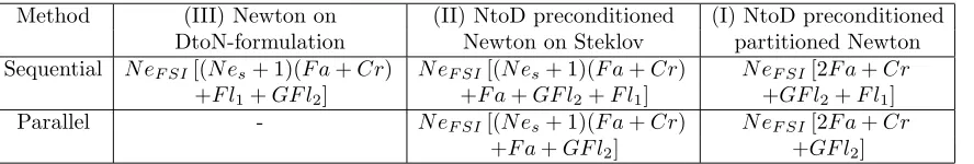
Let us make a formal complexity analysis to have a rough hint on the cost of the Steklov type, Dirichlet to Neumann formulation based, and partitioned Newton type methods. We make the following assumptions: the fluid to be solved at each time step is linear (e.g. semi-implicit Euler for Navier-Stokes), the structure problem is solved by a Newton algorithm and the linearized structure problems by direct methods. We only take into account the factorization for the resolution of the structure sub-problem and consider the matrices as already factorized when dealing with linear domain decomposition methods.
In the following analysis we assume that the number of Newton iterations N eF SI for the global problem
does not depend on the formulation used: (I), (II) or (III). We denote byN es the number of iterations for a
Newton algorithm in the structure problem. The number of GMRES iterations G is assumed not to depend on the algorithm if optimal preconditioners (let say Dirichlet-Neumann) are used. These simplifications allow us to compare the cost of the different methods. In the sequel Cr and F adenote respectively the cost of the construction and factorization a matrix in the solid,F l1the resolution cost per time step of the fluid problem,
andF l2the resolution cost for a tangent fluid problem. The estimations of costs for the three types of methods
Method (III) Newton on (II) NtoD preconditioned (I) NtoD preconditioned DtoN-formulation Newton on Steklov partitioned Newton Sequential N eF SI[(N es+ 1)(F a+Cr) N eF SI[(N es+ 1)(F a+Cr) N eF SI[2F a+Cr
+F l1+GF l2] +F a+GF l2+F l1] +GF l2+F l1]
Parallel - N eF SI[(N es+ 1)(F a+Cr) N eF SI[2F a+Cr
+F a+GF l2] +GF l2] Table 1. Estimation of cost
Let us comment Table 1. For the sequential implementation, the estimations for the method (I) and (II) only differ by the factorization cost of a solid tangent matrix, which is rather small with respect to the whole cost. This is in agreement with the tests performed in [8] where method (II) is shown to be roughly equivalent to method (I) in terms of cost. If our estimation is still valid, the method (III) should be at least as efficient as the first two, especially if the structure is nonlinear and expensive. On the contrary, ifF l≥F a+Cr then the parallel implementations of methods (II) and (III) seem to be completely equivalent in terms of cost, which is only determined by the fluid. For the parallel implementation, the cost reduction strongly depends on the number of GMRES iterations, and the method (III) still seems to compete with method (II).
The condition F a+Cr ≥ F l is almost never satisfied if classical shell elements are used. However, this condition may be satisfied when 3D shell elements are used to model more realistic constitutive laws for the structure (see [14]). Let consider for instance a mesh with 38000 nodes in the fluid (let say 150000 degrees of freedom). For MITC4 shell elements, we then have 3300 nodes and 16500 degrees of freedom. Preliminary tests show that in this case, with the same computer, F l ≃45s, F a≃0.7s and Cr ≃ 1.7s. Let now consider 3D shell elements (hexahedra, 27 nodes per element) on the same mesh. The number of nodes for the structure increases from 3300 to 22100, and the number of degrees of freedom from 16500 to 66300. The costs for the solid are nowF a≃13sandCr≃50s. We are thus in the situationCr+F a≥F land F l≥F a.
5.
Preliminary numerical results
As a first benchmark test (see [20]), we consider a simplified version of the coupled problem on a simple geometry, and we briefly compare the results with the nonlinear Domain Decomposition method (II). Let Ω be a cylinder of radius R0 = 0.5cm and of length L = 5cm. We use a coarse mesh, made of 4800 tetraedra
(3916 degrees of freedom) for the fluid, and 40 hexaedra (1584 degrees of freedom) for the structure. We set ∆t = 10−4s. The structure is modeled by 3D-shell elements (see [4–6]) with a Saint Venant-Kirchhoff
constitutive law and the physical parametersE= 3·106dynes/cm2,ν= 0.3 andρ
s= 1.2g/cm3. The thickness
of the shell is h = 0.1cm. In particular we use a Q2-finite element with 27 nodes combined with a MITC interpolation rule in the thin direction of the hexaedra. These elements allow us to easily use three dimensional constitutive laws while keeping a reasonable cost (only one layer of elements is necessary). The fluid we consider is driven by the Navier-Stokes equation on a fixed domain (in particular we skip the ALE formulation in this simple test), with µ = 0.03poise and ρf = 1g/cm2. Initially, the fluid is at rest and an over pressure of
1.3332·104dynes/cm2 (10mmHg) has been imposed at the inlet for 0.005s. As expected, a propagation of the
pressure wave is observed and comparable with more classical shell elements.
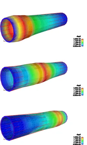
On Figure 2, we plot the deformation of the structure at times 4, 8 and 13ms.
Z X
Y
Z X
Y
Z X
Y
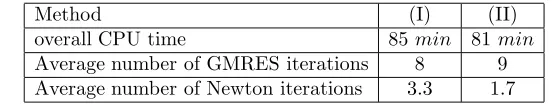
Method (I) (II) overall CPU time 85min 81min Average number of GMRES iterations 8 9 Average number of Newton iterations 3.3 1.7
Table 2. Preliminary numerical results, 150 time steps on the coarse mesh
6.
Conclusion
We have proposed a Newton algorithm for fluid-structure problems. The starting point of the method is the same as for the so-called monolithic approaches since we consider the global fluid-structure equations, but the tangent problem is solved with domain decomposition techniques. The resulting method is therefore partitioned: it is based on two different solvers for the fluid and the structures and can be parallelized. A simplified complexity analysis shows in which cases the proposed method could be competitive. More extensive numerical simulations and comparison with existing methods will be presented in a forthcoming work [14].
References
[1] K.J. Bathe and H. Zhang. Finite element developments for general fluid flows with structural interactions.Int. J. Num. Meth. Engng., 2004.
[2] J.T. Batina. Unsteady Euler airfoil solutions using unstructured dynamic meshes.AIAA J., 28(8):1381–1388, 1990.
[3] P. Causin, J.-F. Gerbeau, and F. Nobile. Added-mass effect in the design of partitioned algorithms for fluid-structure problems. Comp. Meth. Appl. Mech. Engng., 194(42–44):4506–4527, 2005.
[4] D. Chapelle and A. Ferent. Modeling of the inclusion of a reinforcing sheet within a 3D medium.Math. Models Methods Appl. Sci., 13(4):573–595, 2003.
[5] D. Chapelle, A. Ferent, and K.J. Bathe. 3D-shell elements and their underlying mathematical model.Math. Models Methods Appl. Sci., 14(1):105–142, 2004.
[6] D. Chapelle, A. Ferent, and P. Le Tallec. The treatment of ”pinching locking” in 3D-shell elements. M2AN Math. Model. Numer. Anal., 37(1):143–158, 2003.
[7] S. Deparis. Numerical Analysis of Axisymmetric Flows and Methods for Fluid-Structure Interaction Arising in Blood Flow Simulation. PhD thesis, EPFL, Switzerland, 2004.
[8] S. Deparis, M. Discacciati, G. Fourestey, and A. Quarteroni. Fluid-structure algorithms based on Steklov-Poincar´e operators. Comput. Methods Appl. Mech. Engrg., 195(41-43):5797–5812, 2006.
[9] S. Deparis, M. Discacciati, and A. Quarteroni. A domain decomposition framework for fluid-structure interaction problems. InProceedings of the Third International Conference on Computational Fluid Dynamics (ICCFD3), 2004.
[10] W. Dettmer and D. Peri´c. A computational framework for fluid-structure interaction: Finite element formulation and appli-cations.Comp. Meth. Appl. Mech. Engrg., 195(41-43):5754–5779, 2006.
[11] J. Don´ea, S. Giuliani, and J. P. Halleux. An arbitrary Lagrangian-Eulerian finite element method for transient dynamic fluid-structure interactions.Comp. Meth. Appl. Mech. Engng., pages 689–723, 1982.
[12] C. Farhat, K. van der Zee, and Ph. Geuzaine. Provably second-order time-accurate loosely-coupled solution algorithms for transient nonlinear aeroelasticity.Comp. Meth. Appl. Mech. Engng., 195(17-18):1973–2001, 2006.
[13] M. A. Fern´andez and M. Moubachir. Numerical simulation of fluid-structure systems via Newton’s method with exact Jacobians. In P Neittaanm¨aki, T. Rossi, K. Majava, and O. Pironneau, editors,4th
European Congress on Computational Methods in Applied Sciences and Engineering, volume 1, Jyv¨askyl¨a, Finland, July 2004.
[14] M.A. Fern´andez, J.-F. Gerbeau, A. Gloria, and M. Vidrascu. A partitioned Newton method for the interaction of a fluid with a 3D shell structure. In preparation.
[15] M.A. Fern´andez, J.-F. Gerbeau, and C. Grandmont. A projection algorithm for fluid-structure interaction problems with strong added-mass effect.C. R. Acad. Sci. Paris, Math., 342:279–284, 2006.
[16] M.A. Fern´andez, J.-F. Gerbeau, and C. Grandmont. A projection semi-implicit scheme for the coupling of an elastic structure with an incompressible fluid. Int. J. Num. Meth. Engng. in press, 2006.
[17] M.A. Fern´andez and M. Moubachir. An exact block-Newton algorithm for solving fluid-structure interaction problems.C. R. Math. Acad. Sci. Paris, 336(8):681–686, 2003.
[19] M.A. Fern´andez and M. Moubachir. A Newton method using exact Jacobians for solving fluid-structure coupling.Comp. & Struct., 83:127–142, 2005.
[20] L. Formaggia, J.-F. Gerbeau, F. Nobile, and A. Quarteroni. On the coupling of 3D and 1D Navier-Stokes equations for flow problems in compliant vessels.Comp. Meth. Appl. Mech. Engrg., 191(6-7):561–582, 2001.
[21] J.-F. Gerbeau and M. Vidrascu. A quasi-Newton algorithm based on a reduced model for fluid-structure interactions problems in blood flows.Math. Model. Num. Anal., 37(4):631–648, 2003.
[22] M. Heil. An efficient solver for the fully coupled solution of large-displacement fluid-structure interaction problems.Comput. Methods Appl. Mech. Engrg., 193(1-2):1–23, 2004.
[23] B. H¨ubner, E. Walhorn, and D. Dinkle. A monolithic approach to fluid-structure interaction using space-time finite elements. Comp. Meth. Appl. Mech. Engng., 193:2087–2104, 2004.
[24] P. Le Tallec. Domain decomposition methods in computational mechanics. In Computational Mechanics Advances, Vol. 1, no.2, pages 123–217. North Holland, 1994.
[25] P. Le Tallec and J. Mouro. Fluid structure interaction with large structural displacements.Comput. Meth. Appl. Mech. Engrg., 190:3039–3067, 2001.
[26] D. P. Mok and W. A. Wall. Partitioned analysis schemes for the transient interaction of incompressible flows and nonlinear flexible structures. In K. Schweizerhof W.A. Wall, K.U. Bletzinger, editor, Trends in computational structural mechanics, Barcelona, 2001. CIMNE.
[27] D. P. Mok, W. A. Wall, and E. Ramm. Partitioned analysis approach for the transient, coupled response of viscous fluids and flexible structures. In W. Wunderlich, editor,Proceedings of the European Conference on Computational Mechanics. ECCM’99, TU Munich, 1999.
[28] D. P. Mok, W. A. Wall, and E. Ramm. Accelerated iterative substructuring schemes for instationary fluid-structure interaction. In K.J. Bathe, editor,Computational Fluid and Solid Mechanics, pages 1325–1328. Elsevier, 2001.
[29] F. Nobile.Numerical approximation of fluid-structure interaction problems with application to haemodynamics. PhD thesis, EPFL, Switzerland, 2001.
[30] S. Piperno, C. Farhat, and B. Larrouturou. Partitioned procedures for the transient solution of coupled aeroelastic problems. Part I: Model problem, theory and two-dimensional application.Comp. Meth. Appl. Mech. Engrg., 124:79–112, 1995. [31] S. Rugonyi and K.J. Bathe. On finite element analysis of fluid flows coupled with structural interaction. CMES - Comp.
Modeling Eng. Sci., 2(2):195–212, 2001.
[32] T.E. Tezduyar. Finite element methods for fluid dynamics with moving boundaries and interfaces.Arch. Comput. Methods Engrg., 8:83–130, 2001.
[33] P.D. Thomas and C.K. Lombard. Geometric conservation law and its application to flow computations on moving grids.AIAA J., 17(10):1030–1037, 1979.
[34] J. Vierendeels. Implicit coupling of partioned fluid-structure interaction solvers using reduced order models. In M. Sch¨afer H.J. Bungartz, editor,Fluid-Structure interaction, Modelling, Simulation, Optimization, pages 1–18. Springer, 2006. [35] H. Zhang, X. Zhang, S. Ji, G. Guo, Y. Ledezma, N. Elabbasi, and H. deCougny. Recent development of fluid-structure