88 Trans. Phenom. Nano Micro Scales, 7(2): 88-96, Summer and Autumn 2019
DOI: 10.22111/tpnms.2019.28478.1170
DOI: 10.
Numerical Simulation of Turbulent Subsonic Compressible Flow through
Rectangular Microchannel
Reza Abdollah pour Malakshah1, Mehdi Mohseni2,*
1MSc, Department of Mechanical Engineering, Qom University of technology, Qom, Iran
2Assistant professor, Department of Mechanical Engineering, Faculty of Engineering, Qom University of technology, Qom, Iran, P.O.B. 1519-37195
Received 16 January 2019; revised 4 June 2019; accepted 6 June 2019; available online 29 July 2019
ABSTRACT: In this study, turbulent compressible gas flow in a rectangular micro-channel is numerically investigated. The gas flow assumed to be in the subsonic regime up to Mach number about 0.7. Five low and high Reynolds number RANS turbulence models are used for modeling the turbulent flow. Two types of mesh are generated depending on the employed turbulence model. The computations are performed for Reynolds number up to 19000 and two inlet pressures of 1102 kPa and 499 kPa. The longitudinal variations of flow characteristics such as pressure, temperature, Mach number and friction factor are investigated. The experimental data are also used for the sake of comparison and to find which turbulence model has the best performance. The results show that the turbulence models with wall functions have generally better agreement with the experimental data than those one without wall function. The numerical results are different for normal size pipe flow.
KEYWORDS: Compressible flow; microchannel; numerical simulation; turbulence models
INTRODUCTION
One of the main techniques in the enhancement of heat transfer during recent decades is utilization of micro-channels. Some examples are the use of micro heat exchangers, micro heat sinks and micro-reactors [1-2]. The analysis of flow characteristics in micro-channels have been the subject of a large amount of experimental and numerical studies. One of the main questions in this regard is that under what conditions the macroscale rules for fluid flows are valid for microscale size. Chen and Kuo [3] solved the turbulent flow in normal and micro channels with a numerical method. They used the Baldwin- Lomax turbulence model in their solution and compared the numerical results for friction factor with experimental data as well as Blusius’s equation. Based on their results for normal size tube the calculated friction factor agrees with Blusius’s equation, while it is greater than both Blusius’s equation and the experimental data for micro channels. Murakami [4] investigated the effect of compressibility on friction factor in laminar and turbulent flow in micro-tubes. He found that in turbulent flow the ratio of Darcy-Weisbach friction factor, fD, to corresponding value in incompressible flow as a reference, is a function of Mach number, while this ratio approximately equals to one for Fanning friction factor.Matsushita et al. [5] examined the turbulent gas flow through a micro-tube with hydraulic diameter of 146.76 µm. Their results show that due to compressibility effect the fD is different from Blusius’s equation while the fF agrees with it. Yang et al. [6] investigated the compressible
*Corresponding Author Email: [email protected]
Tel.: +982536641601; Note. This manuscript was submitted on January 16, 2019; approved on June 4, 2019; published online July 29, 2019.
gas flow through heated commercial microtubes. They reported that the heated gas increases the friction factor and its effect becomes greater in smaller tubes.
Turner et al. [7] conducted experiments to investigate the gas flow in microchannel. The gases included the N2, He, and air which flowed in a micro channel with 5-96 µm hydraulic diameter. Their results show that at Ma number 0.35, the compressibility leads to an increase of 15 percent in the friction factor.
Hong et al. [8] experimentally examined the laminar, transitional and turbulent gas flow in microchannels for various hydraulic diameters. They measured the local Ma number as well as local friction factor for the range 58<Re<7965. Their results show that the Darcy friction factor with flow acceleration loss is higher than the Fanning friction factor for both laminar and turbulent flow. In other words, for turbulent flows, the values of Fanning factor coincides with Blasius’s relation, while Darcy factor is higher than it.
Kawashima and Asako [9] used experimental data for friction factor in compressible flow inside micro-channels, suggested an equation for the calculation of gas temperature in the channel length. Based on this equation, they calculated the friction factor for adiabatic flow.
89 Nomenclature
T Temperature (K)
A surface area (m2) u,v velocity components in x and y direction (m/s)
d pipe diameter (m) uτ friction velocity (m/s)
Dh hydraulic diameter of the noncircular duct (m) x axial direction of flow (m)
fd Darcy-Weisbach friction factor y
+
non-dimensional distance from the wall (y+= ρuτ y/µ)
ff Funning friction factor Greek Symbols
g gravitational acceleration (m/s2) ε dissipation rate of k (m2/s3)
H enthalpy (J/kg) λ mean free path of molecules (m)
k turbulent kinetic energy (m2/s2) μ molecular viscosity (kg/m.s)
Kn Knudsen number μt eddy or turbulent viscosity (kg/m.s)
L characteristics length (m) ρ Density (kg m-3)
Ma Mach number τ shear stress (N/m2)
p pressure (N/m2) Subscripts
Prt turbulent Prandtl number (Prt=νt/αt) LRN Low Reynolds Number
q Heat flux (W/m2) RSM Reynolds Stress Model
Q heat transfer rate (W) SKE Standard k-ε model
̇ internal Heat Source (W/m3) SKO Standard k-ω model
Re Reynolds number (Re=ρVD/µ)
It is also observed that the value of critical Reynolds number is between 1500 and 1700.
Rovenskaya [11] computationally studied the 3D rarefied laminar compressible gas flow in microchannel include a 90 bend with first order slip boundary condition. It is found that the inclusion of a bend in a micro-channel enhances mass flow rate, while, it has a local effect and weakly affected the global performance of the channel. In other words, it turn out to be quite similar to those of a straight channel. On the other hand, the slip boundary condition has noticeable effect on the global channel performances where its disregarding can leads to totally misleading results. Hong et al. [12] conducted various experiments on turbulent gas flow through rectangular microchannels with hydraulic diameter of 146.76 µm and 203 µm. They measured the friction factor with constant wall temperature and adiabatic flow boundary conditions. Their results show that for adiabatic boundary condition, the Fanning friction factor agrees with the Blusius’s relation, while it has lower values for the case with constant temperature at the wall. Hong et al. [13] in a new work, suggested an equation for the calculation of average friction factor for gas flow through adiabatic micro-channels. Their results show that the suggested equation is in good agreement with Moody diagram.
Hong and Asako [14] numerically investigated the convective heat transfer of unchoked and choked gas flow in micro-tubes for both laminar and turbulent ideal gas flows. The numerical methodology is based on the Arbitrary- Lagrangian-Eulerian (ALE) method. The Lam-Bremhorst Low-Reynolds number turbulence model was used for turbulent flow in a two-dimensional geometry. They proposed a correlation for the prediction of the heat transfer rate of the unchoked and choked gas flow in micro-tubes.
Yang et al. [15] investigated the effects of compressibility on forced convection of subsonic gas flow in microtubes with different internal diameters by combining experimental data with numerical simulations. They used the Lam–Bremhorst Low–Reynolds number turbulence model in their numerical solution. Their results show that compressibility effects can significantly enhance convective heat transfer when the gas flow is heated at the walls. This enhancement is more remarkable for microtubes with smaller diameters (lower than 200 µm). Also, the conventional correlations for normal size ducts can be used for gas flow through microtubes when the compressibility effect is not significant.
90 Li et al [19] investigated the heat transfer and pressure loss of air turbulent flow in channels with miniature structured ribs on one wall. They applied both experimental and numerical methods and used a LRN k-ε turbulence model in the numerical solution with air having constant properties. The experiments show that the W-ribbed channel leads to the globally averaged Nusselt numbers, overall Nusselt numbers and friction factors of 2.2–2.6, 2.9–3.3 and 2.5–3.7 times those of a smooth channel, respectively, which are higher than those of the V-ribbed channel.
As reported above, studies on the turbulent compressible gas flow through micro-channels needs further investigations especially in the numerical simulations. These studies, usually focused on the calculation of friction factor, Nusselt number, compressibility effect and slip boundary condition. It seems that some shortcomings in this regard which lead to discrepancies with experiments are due to the employed turbulence models. It should be noted that, numerous turbulence models are suggested so far, but they are valid only for a specific range of flow conditions. In this study, several RANS turbulence models, which usually applied in the CFD simulations, are used to simulate the turbulent compressible gas flow in a microchannel. The reason for this is that the performance of these models is investigated for the above mentioned conditions. These models include both low and high Reynolds turbulence models. The solution is carried out as 3D in a rectangular micro channel.
GEOMETRY AND FLOW CONDITIONS
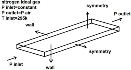
The schematic of the flow geometry and related boundary conditions are shown in Figure 1.
Fig. 1. The schematic of the flow geometry and boundary conditions
The height, width, and the length of the micro channel are based on the experiments of Hong at al [12] and equal to 112.7 µm, 1020 µm and 26.9 mm, respectively. It should be noted that due to the flow symmetry, only one quarter of the geometry has been taken into account, as shown in Figure 2. Thus, the equations are solved in a three-dimensional Cartesian coordinate system. The uniform pressure is used as the inlet and outlet boundary conditions. The flow is considered to be adiabatic, i.e. zero heat flux is assumed as the wall thermal boundary condition.
Fig. 2. Domain Cross section to be considered for numerical simulations
GOVERNING EQUATIONS
In order to determine the flow regime in micro channels, the Knudsen number, Kn, is used. The Kn implies the rarefaction of gas flow and defined as the ratio of mean free path of molecules, λ, to characteristic length of the flow geometry, L, as follows [20].
(1)
In the case of a rectangular microchannel the characteristic length is considered to be the hydraulic diameter (Dh). The mean free path for N2 gas is 0.066 µm and the characteristic length of the micro channel is Dh =203 µm in the current study.
As a result, the Kn equals to 0.000325 which is less than 0.001. This means that the regime of the flow can be considered as continuous. Thus, the Navier-Stokes equations are valid and the no slip conditions should be applied at the wall. It is also, confirmed with the following relation based on the two flow charactristics of Reynolds and Mach numbers [20].
√
√
(2)
The basic governing equations including the conservations of mass, momentum and energy, together with transport equations modeling the turbulence, are employed to model the flow. For steady flow, the conservation of mass states that
( ̅) (3)
For turbulent flows, using the Reynolds time averaging method, the momentum equation yields to:
( ̅ ̅) ̅ ̅ ( ̅̅̅̅̅) (4)
Where
j
i k
i j t ij ij
j i k
u
u
2
u
2
u u
k
x
x
3
x
3
(5)where the symbols with primes denote the fluctuation components of the corresponding quantities.
91 standard k-ω (SKO), SST k-ω, transition k-kl-ω, and Reynolds stress or RSM model. Some of these models, i.e. SKE and RSM, use the wall functions to calculate the quantities in the near wall region while others use damping functions instead.
All above mentioned models are based on the Reynolds average Navier-Stokes (RANS) approach and have 2 to 7 equations which should be solved separately. The k-ε type models are based on turbulent kinetic energy rate (k) and the rate of its dissipation (ε) which introduced by Launder and Spalding [21], while the k-ω type models consist of turbulent frequency (ω) instead of turbulent dissipation rate which is mainly due to the attempts of Wilcox [22]. The RSM model which is the most complicated model with seven equations in 3D solution, solves one equation for each Reynolds stress and is generally more accurate. The energy equation in terms of temperature will be in the form of
( ) (
)
̇
(6)
For flow conditions of this study, the maximum pressure and temperature of nitrogen gas take places at the inlet of channel which are 1102 kPa and 295 K, respectively. The corresponding critical values for pressure and temperature of N2 are 33.9 kPa and 126.2 K [23]. As a results, the compressibility factor for these conditions becomes Z≈0.99 which approximately equals to 1. Thus, the ideal gas equation of state can be used at the present study as follows.
(7)
In order to calculate the friction factor, the following relation is applied [12].
( ) ̇
(
) ( )
(8)
Moreover, in order to comparison the numerical results the Blusius’s relation for the friction factor is used in addition to the experimental data as follows,
(9)
METHOD OF SOLUTION
In order to solve the governing equations, the ANSYS-FLUENT version 18 is used.
The finite volume method is utilized to discretize the nonlinear equations [24].
Also, the SIMPLE algorithm is applied alongside the staggered grid to simultaneously solve the velocity and pressure equations. In addition, the second order upwind scheme is used to approximate the flow field variables in the discretized convective terms in transport equations. The under-relaxation factors are set to default values in FLUENT. The convergence criteria assumed to be 10-6 for all variables.
MESH INDEPENDENCY
In order to reach grid independency, the solution is obtained for various number of nodes in all directions. The velocity magnitude at section 23.3 mm and at inlet pressure of 1102 kPa, is used as criteria for mesh independency. As mentioned before, two types of turbulence models are used in this study.
In the first type (high Reynolds number models) there exists wall function, while the second type (low Reynolds number models) employs damping function. As a result, the mesh generation is different which are investigated separately as follows.
MODELS WITH WALL FUNCTIONS
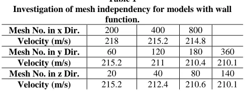
For these models, the mesh generation should satisfy the condition y+>13 [25]. Due to 3D solution, the mesh independency is investigated in three directions separately. In each case, the mesh numbers vary in one direction while are constant in other directions. The results are obtained by using of standard k-ε model and demonstrated in Table 1.
Table 1
Investigation of mesh independency for models with wall function.
Mesh No. in x Dir. 200 400 800 Velocity (m/s) 218 215.2 214.8 Mesh No. in y Dir. 60 120 180 360
Velocity (m/s) 215.2 211 210.4 210.1
Mesh No. in z Dir. 20 40 80 140
Velocity (m/s) 215.2 212.4 210.6 210.1
As expected, by increasing the mesh numbers, the difference between velocity values become smaller. It is concluded that a mesh number of 400*180*80 is a good choice so that increasing the number of grids does not improve the results much further.
MODELS WITHOUT WALL FUNCTIONS
92 For these models a grid numbers of 400*390*100 can be considered as final mesh.
Table 2
Investigation of the mesh independency for models without wall function.
Mesh No. in x Dir. 200 400 600 Velocity (m/s) 195.4 192.3 191.9 Mesh No. in y Dir. 140 280 390 480
Velocity (m/s) 192.3 198.1 199.5 200.1
Mesh No. in z Dir. 50 75 100 125
Velocity (m/s) 187.4 192.3 194.6 195.4
It should be noted that to capture the large variations of flow field variables, a greater number of grids are used close to the wall. It is found by trial and error that the distances between the calculating nodes are most efficient if they grow by a factor of 1.1 as we march away from the wall towards the flow centerline.
RESULTS AND DISCUSSIONS
Based on the experimental data of Hong et al. [12], the simulation was carried out for two inlet pressure of 1102 kPa and 499 kPa at various cross sections listed in Table 3.
Table 3
Sections at which the simulations have been carried out.
Section S1 S2 S3 S4 S5 S6
L(mm) 0 3.3 8.3 13.3 18.3 23.3
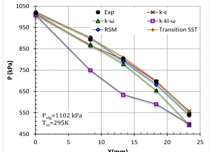
The results for longitudinal variations of pressure in micro-channel length have been shown in Figures 3 and 4 for two inlet pressures, respectively.
Fig. 3. Longitudinal variations of pressure for inlet pressure 1102KPa
The experimental data of Hong et al. [12] are also shown for the sake of comparison. As can be seen, as a result of friction the pressure drops where its variations is not linear due to flow compressibility. It is found that, the RSM model with average errors equal to 0.99 % and 0.8 % has better agreement while the transition k-kl-ω with average error of 12.3 % and 4.99 % has the worst prediction among all other models with respect to the experimental data. The
results of SKE model are also in good agreement with the experiments.
Fig. 4. Longitudinal variations of pressure for inlet pressure 499KPa
In Figures 5 and 6, the variations of gas temperature have been shown for two inlet pressures.
Fig. 5. Longitudinal variations of temperature for inlet pressure 1102KPa
Fig. 6. Longitudinal variations of temperature for inlet pressure 499KPa
220 420 620 820 1020 1220
0 5 10 15 20 25
P
(kPa
)
X(mm)
Exp k-ε
k-ω k-kl-ω
RSM Transition SST
Pstg=1102 kPa
Tin=295K
450 550 650 750 850 950 1050
0 5 10 15 20 25
P
(k
Pa
)
X(mm)
Exp k-ε
k-ω k-kl-ω
RSM Transition SST
Pstg=1102 kPa
Tin=295K
220 270 320 370 420 470 520
0 10 20 30
P
(kPa
)
X(mm)
Exp k-ε
k-ω k-kl-ω
RMS Transition SST
Pstg=499 kPa
Tin=295K
250 260 270 280 290 300
0 10 20 30
T (K)
X(mm)
Exp k-ε
k-ω k-kl-ω
RSM Transition SST
Pstg=1102 kPa
Tin=295K
260 265 270 275 280 285 290 295
0 10 20 30
T (k
)
X(mm)
Exp k-ε
k-ω k-kl-ω
RMS Transition SST
Pstg=499 kPa
Tin=295K
260 265 270 275 280 285 290 295
0 5 10 15 20 25
T(k
)
X(mm)
Exp k-ε
k-ω k-kl-ω
RMS Transition SST
Pstg=499 kPa
93 As a result of pressure reduction in the channel length, the temperature decreases.
In this cases, the RSM and SST k-ω models both with average errors of 0.22 % for pressure 1102 kPa and the SKE model with 0.12 % error for pressure 499 kPa have the best performance while the transition k-kl-ω with average error of 3.12 % and 2.15 % is the worst model to evaluation the experimental data.
The variations of Mach number at two inlet pressures of 1102 kPa and 499 kPa are plotted in Figures 7 and 8, respectively. Similar to velocity, the Ma number increases with channel length.
Fig. 7. Longitudinal variations of Mach number for inlet pressure
1102KPa
As can be seen, the k-ω and the RSM models with average error of 1.9 % and 2.36 % are the best models, respectively. Again, the transition k-kl-ω with error equal to 18.97 % and 20.97 % has the worst prediction of Ma number between all turbulence models against the experimental data.
Fig. 8. Longitudinal variations of Mach number for inlet pressure 499KPa
Based on the applied pressures on two ends of the channel the mass flow rate of gas obtained with various turbulence models are presented in Table 4. As it is
expected, once the pressure difference increases, the mass flow rate grows as well.
Table 4
mass flow rate obtained from various turbulence models.
Turbulence model
Mass Flow Rate (g/s) P=1102 kPa P=499 kPa
k-ε 0.0403 0.0167
k-ω 0.0431 0.0181
k-kl- ω 0.0415 0.0196
RSM 0.0390 0.0160
Transition SST 0.0395 0.0184
FANNING FRICTION FACTOR
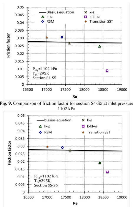
As mentioned before in the introduction, based on the previous studies, the Fanning friction factor i.e. Equation 8, for turbulent flow in microchannels agrees with the famous relation of Blasius. In this study, the friction factor at two segments of S4-S5 and S5-S6 are calculated and compared with Blasius’s relation. Figure 9 to 12 shows the results for two inlet pressures of 1102 kPa and 499 kPa.
Fig. 9. Comparison of friction factor for section S4-S5 at inlet pressure
1102 kPa
Fig. 10. Comparison of friction factor for section S5-S6 at inlet pressure
1102 kPa 0 0.2 0.4 0.6 0.8
0 5 10 15 20 25
Ma
X(mm)
Exp k-ε
k-ω k-kl-ω
RSM Transition SST
0.3 0.35 0.4 0.45 0.5 0.55 0.6 0.65 0.7 0.75
0 5 10 15 20 25
Ma
X(mm)
Exp k-ε
k-ω k-kl-ω
RSM Transition SST
Pstg=1102 kPa
Tin=295K
0 0.2 0.4 0.6 0.8
0 10 20 30
Ma
X(mm)
Exp k-ε
k-ω k-kl-ω
RMS Transition SST
Pstg=499 kPa
Tin=295K
0.25 0.3 0.35 0.4 0.45 0.5 0.55 0.6 0.65 0.7
0 5 10 15 20 25
Ma
X(mm)
Exp k-ε
k-ω k-kl-ω
RMS Transition SST
Pstg=499 kPa
Tin=295K
0 0.01 0.02 0.03 0.04 0.05
16800 17300 17800 18300 18800
Fan n in g Frictio n Fa cto r Re Blasius eq. k-ε
k-ω k-kl-ω
RSM Transition SST
Pstg=1102 kPa
Tin=295K
N2 S4-S5 0 0.005 0.01 0.015 0.02 0.025 0.03 0.035 0.04 0.045 0.05
16500 17000 17500 18000 18500 19000
Fr ict ion f act or Re
Blasius equation k-ε
k-ω k-kl-ω
RSM Transition SST
Pstg=1102 kPa
Tin=295K
Section S4-S5 0 0.01 0.02 0.03 0.04 0.05
16800 17300 17800 18300 18800
Fan n in g Frictio n Fa cto r Re Blasius eq. k-ε
k-ω k-kl-ω
RSM Transition SST
Pstg=1102 kPa
Tin=295K
N2 S5-S6 0 0.005 0.01 0.015 0.02 0.025 0.03 0.035 0.04 0.045 0.05
16500 17000 17500 18000 18500 19000
Fr ict ion fa ct or Re
blasius equation k-ε
k-ω k-kl-ω
RSM Transition SST
Pstg=1102 kPa
Tin=295K
94
Fig. 11. Comparison of friction factor for section S4-S5 at inlet pressure
499 kPa
Fig. 12. Comparison of friction factor for section S5-S6 at inlet pressure
499 kPa
It is found that, the Standard k-ε model with minimum error in all states has the best evaluation while the transition k-kl-ω has the maximum error to predict the friction factor. The details of errors for these two models are listed in Table 5.
Table 5
The error values for the best and the worst predictions for friction factor (percent) in comparison to Blasius’s relation.
Figure 9 Figure 10 Figure 11 Figure 12
SKE model 2.02 0.59 5.87 5.15
k-kl-ω model 197.35 101.93 75.07 112.22
RESULTS FOR NORMAL SIZE PIPE FLOW
In order to further investigate the effect of turbulence model on the compressible flow, in this section, the simulations are performed for a normal size tube with internal diameter of 1 cm and length of 1.35 m. The pressure at the pipe inlet is considered to be 200 kPa and atmosphere at the exit.
The Fanning friction factor for the segment 0.8 m to 1.2 m of the pipe is computed and compared with Blusius’s relation.
The results are shown in Figure 13. As can be seen, the k-ω model has better prediction among other turbulence models while it has at least an error of 10 percent for microchannel.
Again, results of the k-kl-ω model deviates considerably from experimental data. The k-ε model also has a good agreement with the Blasius’s relation.
Fig. 13. Comparison of friction factor for inlet pressure of 200 kPa for
normal size pipe flow
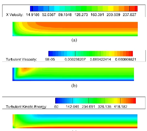
Flow characteristics
In order to better understand the physics of the turbulent flow, in this section, some flow contours are plotted. These includes contours of velocity, turbulent viscosity and turbulent kinetic energy which are shown in Figure 14a, b, and c.
0 0.01 0.02 0.03 0.04 0.05
7000 7500 8000 8500
Fan
n
in
g Frictio
n
Fa
cto
r
X(mm) Blasius eq. k-ε
k-ω k-kl-ω
rsm transition sst
Pstg=499 kPa
Tin=295K
N2
S4-S5
0 0.01 0.02 0.03 0.04 0.05
7000 7500 8000 8500
Fan
n
in
g Frictio
n
Fa
cto
r
X(mm) Blasius eq. k-ε
k-ω k-kl-ω
rsm transition sst
Pstg=499 kPa
Tin=295K
N2
S5-S6
-0.005 0.005 0.015 0.025
170000 175000 180000 185000 190000 195000
f
Re
blasius eq k-ω
k-kl- ω Transition SST
RSM k-ε
Pstg=200 kPa
Tin=295 K
N2
0.8-1.2
(a)
(b)
(c)
Fig. 14. Contours of some turbulent flow characteristics, (a) velocity (m/s),
95 For this reason, the results obtained by the k-ε turbulence model at section L=23.3 mm and at inlet pressure of 1102 kPa are used.
It should be noted that, as mentioned in section two, Geometry and Flow Conditions, due to the flow symmetry only one quarter of the geometry has been considered to be solved, as shown in Figure 2.
As can be seen, the turbulent viscosity has its maximum values near the shorten walls of the channel where the secondary flows are formed.
In the other hand, the maximum of turbulent kinetic energy take places near the walls in in the log-law layer where the velocity variations is large.
CONCLUSIONS
In this study, the subsonic turbulent flow of nitrogen gas is simulated using CFD methods. Five low and high RANS turbulence models are used to model the turbulent flow. The simulations have been carried out using three dimensional model in a rectangular microchannel. The following conclusions may be derived from this study. 1- Generally speaking, the Standard k-ε model with
standard wall function has the best evaluation of flow characteristics such as pressure, temperature and friction factor, among all turbulence models applied. The error for this model is less than 6 percent for all flow conditions.
2- The transition k-kl-ω model without wall function has the largest errors with respect to other turbulence models in comparison to experimental data. The maximum error is greater than 100 percent for some flow conditions, i.e. calculation of friction factor. Thus, this model is not recommended for flow conditions of the present study. This is true for both micro and normal size channels. It seems that this model is not suitable for compressible flow.
3- The Standard k-ω and the transition SST k-ω models without wall function, have generally less precision with respect to k-ε model for compressible flow in microchannels, especially for calculation of friction factor. However, the Standard k-ω model evaluate the friction factor for normal size pipe more accurately.
4- The RSM model has acceptable results for all flow conditions applied here. The maximum error for this model is about 13 % which take places in normal size pipe flow. It has a difference about 9 % with Basius’s relation for micro-channel simulations.
REFERENCES
[1] Xu B, Wong TN, Nguyen NT. Investigation of heat
transfer in a microchannel with same heat capacity
rate. Heat and Mass Transfer. 2019 Mar
8;55(3):899-909.
[2] Sivasankaran S, Narrein K. Influence of Geometry
and Magnetic Field on Convective Flow of Nanofluids in Trapezoidal Microchannel Heat Sink. Iranian Journal of Science and Technology, Transactions of Mechanical Engineering.:1-0.
[3] Chen CS, Kuo WJ. Numerical study of compressible turbulent flow in microtubes. Numerical Heat Transfer, Part A: Applications. 2004 Jan 1;45(1):85-99.
[4] Murakami S, Asako Y. Local Friction Factor of
Compressible Laminar or Turbulent Flow in Micro-Tubes. InASME 2011 9th International Conference on Nanochannels, Microchannels, and Minichannels 2011 Jan 1 (pp. 295-303). American Society of Mechanical Engineers.
[5] Matsushita S, Hong C, Asako Y, Ueno I.
Experimental Investigations of Turbulent Gas Flow through a Micro-tube. InProceedings of the 4th International Conference on Heat Transfer and Fluid Flow in Microscale 2011.
[6] Yang Y, Schakenbos T, Chalabi H, Lorenzini M, Morini GL. Compressible gas flow through heated commercial microtubes. Proceedings of the 4th Int Conference on Heat Transfer and Fluid Flow in Microscale, Fukuoka, Japan. 2011.
[7] Turner SE, Lam LC, Faghri M, Gregory OJ. Experimental investigation of gas flow in microchannel. Int. J. Heat Mass Transf. 2004; 127: 753–763.
[8] Hong C, Yamada T, Asako Y, Faghri M. Experimental investigations of laminar, transitional and turbulent gas flow in microchannels. Int. J. Heat Mass Transf. 2012; 55: 4397–4403.
[9] Kawashima D, Asako Y. Data reduction of friction factor of compressible flow in micro-channels. Int. J. Heat Mass Transf. 2014; 77: 257–261.
[10] Tao Z, Zhu Z, Li H. Experimental investigation of the air flow behavior and heat transfer characteristics in microchannels with different channel lengths. J. Heat Transfer. 2017; 139: 052403-1.
[11] Rovenskaya OI. Computational study of 3D rarefied gas flow in microchannel with 90 bend. Eur. J. Mech. B Fluids. 2016 September–October; 59: 7-17. [12] Hong C, Nakamur T, Asako Y, Ueno I. Semi-local
friction factor of turbulent gas flow through rectangular microchannels. Int. J. Heat Mass Transf. 2016; 98: 643–649.
[13] Hong C, Asako Y, Morini GL, Rehman D. Data reduction of average friction factor of gas flow through adiabatic micro-channels. Int. J. Heat Mass Transf. 2019; 129: 427–431.
96 Nanochannels, Microchannels, and Minichannels. ICNMM2014. Chicago. Illinois: USA. 2014 August.
[15] Yang Y, Hong C, Morini GL, Asako Y.
Experimental and numerical investigation of forced convection of subsonic gas flows in microtubes. Int. J. Heat Mass Transf. 2014; 78: 732–740.
[16] Hong C, Tanaka G, Asako Y, Katanoda H. Flow characteristics of gaseous flow through a microtube discharged into the atmosphere. Int. J. Heat Mass Transf. 2018; 121: 187–195.
[17] Shui L, Huang B, Gao F, Rui H. Experimental and numerical investigation on the flow and heat transfer characteristics in a tree-like branching microchannel. J. Mech. Sci. Technol. 2018; 32 (2): 937-946.
[18] Asako Y, Heng SY, Hong C. On temperature jump
condition for turbulent slip flow in a quasi-fully developed region of micro-channel with constant wall temperature. Int. J. Therm. Sci. 2019; 136: 467– 472.
[19] Li Y, Rao Y, Wang D, Zhang P, Wu X. Heat transfer
and pressure loss of turbulent flow in channels with miniature structured ribs on one wall. Int. J. Heat Mass Transf. 2019; 131: 584–593.
[20] Nicolas X, Chénier E, Tchekiken C, Lauriat G.
Revisited analysis of gas convection and heat transfer in micro channels: Influence of viscous stress power at wall on Nusselt number. Int. J. Therm. Sci. 2018; 134: 565–584.
[21] Launder B, Spalding D. The numerical computation
of turbulent flows. Comput. Methods Appl. Mech. Eng. 1974; 3: 269-89.
[22] Wilcox DC. Simulation of transition with a
two-equation turbulence model. AIAA J. 1994 February; 32 (2): 247-254.
[23] Cengel YA, Boles MA. Thermodynamics, an
engineering approach. 8th ed. New York: McGraw-Hill Education; 2015.
[24] Versteeg HK, Malalasekera W. An Introduction to
computational fluid dynamic, the finite volume method. 2nd ed: Longman Group Ltd. 2007.