Most of the Time, It Works Every Time: Limitations in Refining Domain Models with Learning Curves

(1)

Most of the Time, It Works Every Time:

Limitations in Refining Domain Models with

Learning Curves

Ilya Goldin

2U, Inc.

[email protected]

April Galyardt

Software Engineering Institute [email protected]

Data from student learning provide learning curves that, ideally, demonstrate improvement in student performance over time. Existing data mining methods can leverage these data to characterize and improve the domain models that support a learning environment, and these methods have been validated both with already-collected data, and in close-the-loop studies that actually modify instruction. However, these methods may be less general than previously thought, because they have not been evaluated under a wide range of data conditions. We describe a problem space of 90 distinct scenarios within which data mining methods may be applied to recognize posited domain model improvements. The scenarios are defined by two kinds of domain model modifications, five kinds of learning curves, and 25 types of skill combinations under three ways of interleaving skill practice. These extensive tests are made possible by the use of simulated data. In each of the 90 scenarios, we test three predictive models that aim to recognize domain model improvements, and evaluate their performance. Results show that the conditions under which an automated method tests a proposed domain model improvement can drastically affect the method’s accuracy in accepting or rejecting the proposed improvement, and the conditions can be affected by learning curve shapes, method of interleaving, choice of predictive model, and the threshold for predictive model comparison. Further, results show consistent problems with accuracy in accepting a proposed improvement by the Additive Factors Model, made popular in the DataShop software. Other models, namely Performance Factors Analysis and Recent-Performance Factors Analysis, are much more accurate, but still struggle under some conditions, such as when distinguishing curves from two skills where students have a high rate of errors after substantial practice. These findings bear on how to evaluate proposed refinements to a domain model. In light of these results, historical attempts to test domain model refinements may need to be reexamined.

Keywords:domain model, predictive model, Q-matrix, learning curve

1. I

NTRODUCTION

(2)

For example, when the learning objective is introductory computer programming in Lisp, a domain model should distinguish the sub-skills of defining a first parameter to a Lisp function and of defining subsequent parameters to a function (Corbett and Anderson, 1995). As a second example, when the target domain is a course on algorithms, the intended audience of students has likely long mastered basic programming knowledge. Accordingly, a domain model for this course might reasonably assume that the learner population has a baseline level of programming ability and ignore skill distinctions such as defining first versus subsequent parameters.

A domain model for some target domain can change over time. Because domain models reflect scientific knowledge about how to teach some set of skills, they are subject to revision as scientific understanding improves.1 _{If we treat different plausible domain models for the}

same learning objective as hypotheses about instruction and test them with learners, we may find evidence in support of one domain model over another, and thereby gain new knowledge about how people come to master this objective.

The present work examines whether or not we can be certain that a posited domain model improvement can actually be detected in observed student behaviors. The focus is on assessing the methodology for domain model refinement, not any specific domain model or predictive model.

Intriguingly, we can test domain models against already collected data. Although the in-ferences from such data mining studies are not as strong as from controlled experimentation, they can be implemented for the cost of running a statistical procedure, and as such can be tremendously useful (Martin et al., 2011;Koedinger et al., 2012;Goldin et al., 2016), especially when domain model improvements are non-obvious (Koedinger and McLaughlin, 2016). The methodology has been validated through studies that “close the loop” by identifying candidate domain model refinements on existing data, and then testing a refined domain model with new students (Koedinger et al., 2013).

Data mining studies for domain model improvement are essentially statistical tests. Subject matter experts posit that some feature of the domain ought to be reflected in student practice in the domain, and create two domain models that differ only with respect to the feature in question. Then they compare which of the models more accurately predicts student activity in the extant dataset. Any statistical test comparing predictions from two domain models is necessarily subject to potential false negative and false positive errors. These errors can lead us to choose a domain model that fails to describe some feature of the domain correctly, and therefore give rise to inefficient instruction and inaccurate assessment.

The structure of this paper is as follows. After a review of related work on domain model improvement, the paper formalizes two problem cases: the case that the true domain model contains one skill (i.e., a two-skill split coding is false), or that it contains two skills (a one-skill merge coding is false). Further, data-driven recognition of domain model improvement is complicated by data characteristics, as demonstrated in five distinct types of learning curves and three ways of combining (interleaving) these curves. The following section on research methods defines three tests of domain model improvement, including the original test using the Additive Factors Model (Cen et al., 2006), and alternative tests using the models Performance Factors Analysis (Pavlik Jr et al., 2009) and Recent-Performance Factors Analysis (Galyardt and Goldin, 2015; Goldin and Galyardt, 2015). The section also explains how simulated data 1_{The term}_skill_{in this paper is meant generically, and applies equally to concepts, facts, or other atomic}

(3)

can be used to evaluate these tests. The subsequent sections report and discuss the results of the study. In brief, we find that some data generative conditions are inherently more challenging than others for detecting domain model improvements. Further, we find that the Additive Factors Model has consistent patterns of failing to recognize valid domain model improvements, and that alternative tests are more sensitive. The paper concludes with a discussion of the implications of the results and suggests some directions for future work.

1.1. RELATED WORK

A simple computational representation for a domain model is a Q-matrix (Tatsuoka, 1983). A Q-matrix is a table: each row corresponds to one assessment item in the domain of interest, or a sub-item, such as a step in the solution of a problem; each column corresponds to a latent skill or knowledge component variable hypothesized to matter in the domain; and each table cell contains a (usually binary) value that encodes whether or not some skill is relevant to some assessment item or sub-item. Using this representation, two models for the same domain may differ if they contain different values in one or more cells, or if they contain different columns. A Q-matrix is not the only possible implementation of a domain model. For example, Knowledge Spaces (Falmagne et al., 1990) do not represent the notion of a skill; instead, they represent assessment items and prerequisite relationships among these.

It is possible to try to discover an entire Q-matrix in a data-driven way (Liu et al., 2012;

Desmarais, 2012). By using repeated observations of a learner’s performance on a skill, it is possible to discover a domain model and learn student proficiency parameters at the same time (Gonzlez-Brenes and Mostow, 2013). Nonetheless, it is challenging to understand how loadings on an automatically discovered Q-matrix connect to a curriculum and to human expert understanding of a domain.

One way to bridge data-driven methods and human understanding is to refine an existing Q-matrix rather than learning one from scratch. In domain model refinement, we only need to interpret a change to a Q-matrix (Koedinger et al., 2012). The proposed changes may be human-authored also, such as the “difficulty factor” (Baker et al., 2007), further facilitating interpretability.

Learning Factors Analysis (Cen et al., 2006) automates a heuristic search in a space of Q-matrices, enabling iterative refinement that starts with an existing Q-matrix. LFA consists of three parts: a procedure to search the space of domain models; a set of 3 change operators that may alter a domain model; and a domain model evaluation component, the output of which guides the search. The three change operators are split, merge, and add. The split operator replaces a single latent skill variable in the Q-matrix with two distinct variables, each of which only codes for a subset of the activities that bear on the original latent variable. The merge operator does the reverse, replacing two existing latent variables with a new latent that is their union. The add operator inserts an extra Q-matrix column, creating an additional loading on a latent skill variable without removing any existing loadings. Each posited domain model refinement calls for an application of these operators and necessitates a new comparison to evaluate the modified Q-matrix.

(4)

discriminates between individuals who possess all attributes required for item and individuals who lack one or more required attributes for the item (de la Torre and Chiu, 2016). This index therefore indicates a possible misspecification in the Q-matrix.

Data from test administrations and from tutoring applications differ in significant ways. In most test administrations, by design, we assume that students do not learn during the test, and therefore models of test data can ignore any order effects among multiple assessments of one skill. By contrast, in tutoring data, we hope for learning, and therefore models of these data need to account for temporal effects. In addition to differences in model structure, the assumption that performance on a skill will improve over time provides important information to the tutoring-data models that is not available to test-tutoring-data models, as leveraged in this paper.

Specifically, data from student practice with some set of learning activities can be plotted as a set of learning curves. It is not trivial to plot one curve per skill because of compensatory skill relationships, condensation rules, and credit assignment (Rupp and Templin, 2008). Nonethe-less, given a dataset from student practice that is defined with respect to a domain model, we can plot learning curves: for each skill in the domain model, for each practice opportunity, we can plot the average population probability of success on the skill (or equivalently, the error rate, flipping the vertical axis).

A domain model may represent information beyond the mapping between assessment items and relevant skills. Depending on the instructional setting, a tutoring system may also represent the prerequisite structure, i.e., the dependencies among the skills, which may inform both in-struction and assessment. Prerequisite dependencies may also be learned automatically (Vuong et al., 2011;Scheines et al., 2014;Chen et al., 2016).

A domain model may be brought to bear on predicting student performance. For example, a variety of Linear Logistic Test Models (Fischer, 1973;de Boeck and Wilson, 2004) explicitly incorporate a Q-matrix, including the logistic regression models used in this work, as described inSection 3.4.(Cen et al., 2006;Pavlik Jr et al., 2009;Galyardt and Goldin, 2015). Alternatively, a Bayesian Knowledge Tracing predictive model (Corbett and Anderson, 1995) implicitly uses a Q-matrix by allocating independent parameters for each skill.

The development of predictive models stems from the need for large-scale testing, and is described in decades of psychometric literature. More recently, predictive models have been at the center of literature on educational data mining. One prominent use is to predict whether or not a student will answer a problem correctly, which enables decision-making in tutoring systems (Corbett and Anderson, 1995). This use case has prompted investigations of model variants, of their predictive accuracy and of model errors (Yue et al., 2011; Kser et al., 2014;

Stamper et al., 2013; Galyardt and Goldin, 2015). Predictive models have also been used to connect human learning to domain model refinement (Cen et al., 2006; Martin et al., 2011;

Koedinger et al., 2012;Koedinger et al., 2013).

The structure of a predictive model can represent different conceptualizations of human learning and performance. For example, a population-level view of learning implies that av-erage population performance on some set of tasks ought to improve as the population learns. By contrast, a mastery-disaggregated view of learning (Murray et al., 2013) holds that individual students may engage in practice for some time before demonstrating correct performance (Kser et al., 2014;Galyardt and Goldin, 2015).

(5)

sufficiently evidence the behavior that reflects that aspect of cognition. One standard statistical method to evaluate model validity is to ascertain that the model is capable of estimating its pa-rameters on data that are known to evidence the behavior in question, and one easy way to obtain such data is by simulation, i.e., to ensure the necessary evidence is present by construction. In the case of student learning, one approach is to generate data from a rich cognitive model such as ACT-R (Anderson, 1996) or SimStudent (Matsuda et al., 2015). Another approach focuses not on the latent constructs of the cognitive model but on observable behavior, such as on the process of student activity (Lindsey et al., 2014).

Domain model improvements have multiple uses in tutoring systems, e.g., more accurate re-porting, sequencing problems that pertain to a skill, creating new tasks or refining instructional messages (Koedinger et al., 2013). Additionally, domain models have multiple uses beyond tutoring. In large-scale testing, a domain model can enable detailed diagnostic reporting and accurate summative assessment, including in adaptive testing settings. In Cognitive Task Anal-ysis, a “task list,” which is effectively the set of skills (rows) in a Q-matrix, enables comparison among human expert instructors in terms of what information they fail to communicate to stu-dents (Sullivan et al., 2014). In psychology research, domain models may be used to investigate cognitive hypotheses, such as in comparing a faculty view of cognition against a component view (Koedinger et al., 2016).

Aside from investigating the validity of a posited change, as in this paper, it may be possible to estimate the impact of a posited change, e.g., on student practice in a tutoring system (Cen et al., 2007; Rollinson and Brunskill, 2015; Kser et al., 2016; Gonzalez-Brenes and Huang, 2015). Errors in domain models may have a significant impact on students. When a model is misspecified, over 50% of the students may be assigned substantial extra practice, as demon-strated on simulated data. (Fancsali et al., 2013) When a single latent variable in a Q-matrix improperly represents two distinct skills, practice and assessment on either skill are not distin-guished from practice and assessment on the other. A student might master one of the two skills, but a tutoring system may miss the mastery and assign extraneous practice, or, conversely, grad-uate the student prematurely from studying one skill because of mastery of the other. When two latent variables improperly represent the same skill, the student may be obligated to demonstrate mastery of multiple (unnecessarily split) skills, slowing down instruction and increasing student effort.

Some published domain model investigations result in domain model expansion, while oth-ers retain a parsimonious domain model. Decisions to split a skill, add a new skill or merge two skills directly affect the practice of future students. As a first example, in geometry, students may struggle with composite area problems, where “the area of a composite shape must be found by combining (adding or subtracting) the areas of two constituent regular shapes (e.g., what’s left when a circle is cut from a square)” (Koedinger et al., 2013, p. 423). The researchers posited that a subset “of the composite problems were ‘scaffolded’ such that they included columns that cued students to find the component areas first.” (Ibid.) As a revised domain model, problems that had been tagged with one column of the Q-matrix were re-tagged with one of three new columns: “one representing ‘compose-by-addition’ with scaffolding present, a second where the student had to ‘decompose’ a composite area without scaffolding, and a third where the stu-dent needs simply to ‘subtract’ in order to execute a decomposition plan.” (Ibid.) This split was validated both in terms of predictive accuracy and in an experiment with students (Koedinger et al., 2013).

(6)

expan-sion was not justified. In a dataset of student practice in computing the area of various simple, non-composite shapes, it was theorized that finding forward computation (e.g., find the area of a circle given the radius) may be distinct from backward computation (find the radius given the area). In this case, predictive accuracy only improved by recoding circle-area problems. Anal-ogous recoding for other shapes, including triangle, trapezoid, etc., did not improve predictive accuracy (Koedinger et al., 2012). Therefore the single skill coding for forward and backward computation of area was selected as the better domain model.

2. P

ROBLEM

S

TATEMENT

We aim to determine whether or not a method is capable of accurately and consistently recog-nizing true domain model improvements. Our research questions are: How often do predictive models fail to recognize improvements to a domain model, under what conditions are these errors likely, and do these conditions vary across the predictive models?

This section describes three factors that can affect the accuracy of recognizing domain model improvements. These include the structure of the underlying generative domain model, the shapes of learning curves for the skills in question, and the order in which students see problems from these skills.

Additional factors may also affect the accuracy of recognizing improvements, including sam-ple size and levels of noise in the data. A comprehensive investigation of these issues is beyond the scope of our analysis, although we make a preliminary investigation of sample size.

2.1. STRUCTURE OF THEGENERATIVEDOMAIN MODEL

As mentioned underSection 1.1., student practice in geometry problem solving is at times better represented by a relatively rich domain model, and on other occasions by using a relatively parsimonious model (Koedinger et al., 2012;Koedinger et al., 2013). As in these examples, the simplest domain model refinement possible is to decide whether a particular set of problems is better modeled by a single skill or a pair of skills.

Accordingly, an automated procedure that recognizes domain model refinements must be evaluated in two ways. Suppose that we could know the true, unobservable domain model underlying a dataset of student practice. When the data arise from a domain model with a single skill, does the procedure correctly select the single skill domain model? When the data is generated by a domain model with two skills, does the procedure correctly select the two skill model? It is important to evaluate an automated refinement recognition procedure in both ways, because a procedure may be biased to reward either expansive or parsimonious domain models. For example, a predictive model that overfits the data would tend to value expansive domain models more often than justified.

2.2. LEARNINGCURVE SHAPES2

(7)

2 4 6 8 10 12 14

0.0

0.2

0.4

0.6

0.8

1.0

Good

Practice Opportunity

% correct

2 4 6 8 10 12 14

0.0

0.2

0.4

0.6

0.8

1.0

High Error

% correct

2 4 6 8 10 12 14

0.0

0.2

0.4

0.6

0.8

1.0

Slow Learning

% correct

2 4 6 8 10 12 14

0.0

0.2

0.4

0.6

0.8

1.0

Already Mastered

% correct

2 4 6 8 10 12 14

0.0

0.2

0.4

0.6

0.8

1.0

Negligible Learning

% correct

(8)

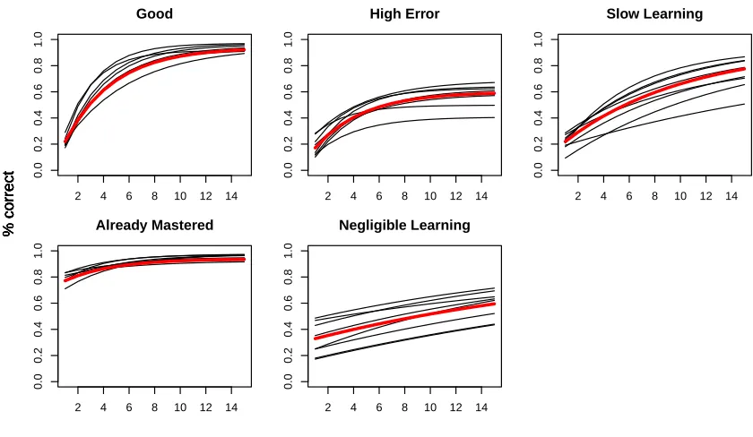
In a Good curve (Figure 1, top left) we observe somewhat idealized student behavior. On early attempts, the percentage of students who answer correctly is fairly low, indicating that the majority of students have yet to master the skill. After some sensible amount of practice, the proportion of students who answer correctly is high, indicating learning.

The High Error curves (Figure 1, top center), represent skills where students have a high probability of making an error despite correct knowledge (i.e., there is a high slip rate for the skill). For example, in basketball there is a low error rate for a free throw, but a three-point shot has an inherently higher error rate as it is taken from a longer distance and opponents are free to move around, and this remains true even for highly skilled players. Assessment of High Error skills must account for this slip rate.

If the population error rate declines slowly (Figure 1, Slow Learning), or almost not at all (Figure 1, Negligible Learning), students may need many practice opportunities to master the skill. Potentially, one curve might in fact be a mixture of two skills, and averaging the skills together obscures the distinct error rates on the two skills. This may indicate an opportunity to revise instruction on this skill, or to consider whether there may be sub-skills that can be called out for targeted instruction and assessment. Alternatively, a Slow Learning skill may just be a skill that takes many more repetitions to master than the idealized Good skills.

When the population error rate is low even at early practice opportunities (Figure 1, Already Mastered), the data indicate that by the time the observed students encountered these activities, they must have already mastered the skill in question.

The learning curve shapes described above are similar but not identical to the curves in the PSLC DataShop (DataShop Team, 2016). In brief, the Good curve type is similar in both settings. The DataShop “low and flat” curve is comparable to Already Mastered in this paper. The DataShop “still high” curve is replaced by two distinct shapes: Slow Learning shows that students may need additional opportunities for practice, and High Error shows that the task is inherently difficult or has a high slip rate, and even additional practice may not reduce error over the long run. Finally, the DataShop “no learning” shape is replaced by Negligible Learning, which still represents that students fail to acquire mastery over time, but allows for a modest aggregate population improvement in performance.

2.3. STRUCTURE OF STUDENTPRACTICE

Consider again the examples fromKoedinger et al. (2013) andKoedinger et al. (2012) refining the domain model in high school geometry. These studies were conducted on already collected data. The students encountered problems according to a structure determined by the domain model at that time. When a new domain model is proposed, the structure of practice for the new skill(s) is different.

(9)

Blocked, even and gradual modes of interleaving, which provide structure to this analysis, are not necessarily tools that are purposefully applied in domain modeling. Comparing these three interleaving regimes to any real-world systems would be beside the point. Rather, de-velopers of a tutoring system may focus on practical concerns when creating domain models, such as limiting the expected amount of student effort (Lee and Brunskill, 2012), and a side effect of that may be some kind of interleaving of skills. Nonetheless, the interleaving regimes circumscribe the continuum of how falsely merged curves might be shaped.

One historically important example for learning curve analysis demonstrates an interleaving of two curves, corresponding to the rule for the first argument and the rule for subsequent ar-guments to a Lisp function (Corbett and Anderson, 1995, Figures 5-6). The curve for the rule pertaining to the first argument, with a first-opportunity error rate of30%and subsequently

ap-proaching virtually no error after practice, is closest to our category of Already Mastered curves. The curve for the rule on additional arguments, with a first-opportunity error rate of55% and

approaching no error after practice, most closely matches the category of Good curves. The second curve begins at practice opportunity 6 relative to the first curve, suggesting that the curve overlap resembles gradual interleaving more so than blocked or evenly interleaved practice.

2.3.1. Generative Model with Two Skills

In the case that the true domain model contains two skills, and a posited domain model inappro-priately tags their items with only one skill, the practice opportunities must be ordered somehow in the merged skill. The Blocked, Even, and Gradualinterleaving regimesdescribed above pro-vide a useful structure to explore the ordering effects of a domain model incorrectly merging what should be two distinct skills.

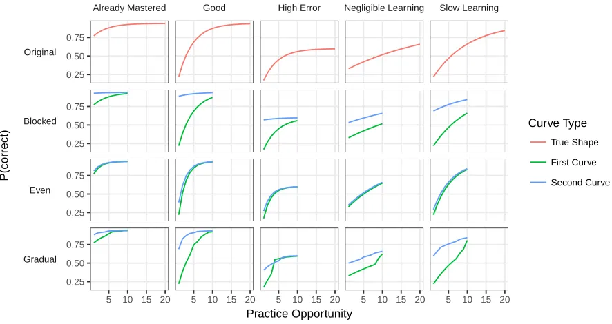
Figure 2 shows what the learning curve for the new single-skill candidate looks like for when both generative skills have a Good curve shape. Under Blocked practice, students com-plete practice on one skill before encountering the second skill; and the learning curve for an inappropriately merged skill will have a dip in the success rate when students begin to practice the second skill (Figure 2Blocked). In Even interleaving (where students practice one activity from each of the skills, then a second activity from each of the skills, etc.), the merged curve is reasonably smooth (Figure 2Even). It is not clear that applying the LFA split operator to such a curve would result in a statistically detectable difference. Under Gradual interleaving, practice on one skill mostly happens first, practice on the second skill mostly happens last, and the skills overlap in the middle of practice. This leads to several smaller dips in the incorrectly merged curve as opposed to the single large dip in the Blocked case. Note thatFigure 2shows the case when both generating curves are type Good; for other curve shapes, the combined curves have similar structure, but the dips may be smaller or larger (Figure 8–Figure 10).

2.3.2. Generative Model with One Skill

(10)

blocked even gradual

5 10 15 20 5 10 15 20 5 10 15 20

0.2 0.4 0.6 0.8

Practice Opportunity (Two Good Skills)

P(correct)

Figure 2: Improperly combined learning curves when practice on two identical, prototypical Good skills is blocked, evenly interleaved, or gradually interleaved

Already Mastered Good High Error Negligible Learning Slow Learning

Original

Blocked

Even

Gradual

5 10 15 20 5 10 15 20 5 10 15 20 5 10 15 20 5 10 15 20

0.25 0.50 0.75

P(correct)

Curve Type

True Shape

First Curve

Second Curve

(11)

highly similar. Lastly, in the Gradual case, the beginning part of the generating curve is mostly allocated towards one skill, and the ending of the generating curve is mostly allocated towards the second skill, but the resulting curves are more jagged than observed in the Blocked case (Figure 3, Gradual row).

In sum, learning curve shape may reveal opportunities for improving the domain model, but it can also hide distinct underlying skills, or it might be improperly split off from another skill. The shapes of an improperly combined curve or improperly separated curves are necessarily af-fected by the mechanism of interleaving practice. Some combinations of curves and interleaving mechanisms may be especially challenging for computational methods of testing proposed splits and merges, i.e., curve shape combinations may vary in the rates of errors that they induce.

3. M

ETHODS

We aim to evaluate the methodology of automated recognition of domain model improvements, and to describe the conditions under which the automated procedure commits errors. Although domain models are inherently unobservable, we have access to the ground truth for our domain model because we create a synthetic dataset, thereby controlling the domain model, the skill properties and the interleaving (for one true skill) or sampling (for two true skills) method.

We use simulated data so that, by construction, we can know whether the correct model is the original or the proposed modification. By contrast, it is difficult to know the ground truth regarding a domain model in data collected from human learners, because domain models are unobservable, latent variables, they are designed by fallible human experts, and noise in human performance data can muddy the waters. Even in trivially simple or artificial domains, noise may arise because individual learners pursue distinct problem-solving strategies and shift strategies over time (Anderson, 2013;Galyardt, 2012).

Moreover, simulated data heads off methodological confounds. First, when working with real data, we conventionally rely on a statistical procedure to tell us whether a particular domain model refinement is an improvement. In this paper, it is that very statistical procedure we wish to evaluate. Suppose that, for a given real-world dataset, we could achieve similar predictive accuracy by positing a richer domain model, or by positing a richer model of student proficiency with a basic domain model. Should we believe that the richer domain model or the basic one is closer to the true model?

Second, the questions pertain to interactions of factors, such as recognizing when a single learning curve should be split into two, where the component curves have particular shapes, and when they are interleaved in a particular way. Such interactions are the focus of our analysis, but they are infrequent events in data from human learners. Simulation allows for an unlimited quantity of data, enabling accurate, reliable measurement.

As described above, we consider 2 generative domain models (single-skill and two-skill), 5 learning curve shapes, and 3 modes of interleaving. The two-skill generative case, by definition, contains 2 true curves, with 5 options for the first curve and 5 options for the second, yielding

5_×5_×3 = 75scenarios. In the single-skill case, there’s one true curve shape, yielding5_×3 = 15

scenarios.

(12)

dataset corresponding to the simulation condition. Each skill is practiced by 100 simulated students, who make an average of 10 attempts per skill, or more precisely pi attempts, where

pi ∼ P oisson(10). We chose a mean of 10 opportunities for each person for each skill, as a best-case realistic scenario - it is near the average number observed per skill in many real datasets. The secondary dataset is then combined with the primary dataset. In each of the 90 scenarios, the simulation is repeated 500 times.

3.1. SIMULATING DATA FROM LEARNINGCURVE ARCHETYPES

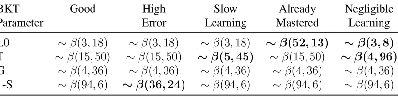
We use Bayesian Knowledge Tracing (BKT) to synthesize both the primary and secondary datasets (Corbett and Anderson, 1995;Reye, 2004). BKT does not represent the complex detail of human cognition, but it is useful to treat it as an idealized, abstract model of observable stu-dent behavior. (BKT’s limitations and some alternative models are discussed underSection 5.4.). Given that we are testing whether refinements to the domain model are detectable, we do not have to assume that the generating model is “correct.” We merely need a method for generating correct and incorrect responses by synthetic students that maps well to the learning curve shapes defined inSection 2.2..

BKT is a Hidden Markov Model with four parameters and manipulating these four parame-ters produces curves in each archetypal learning curve shape.

• L0, the probability of having already mastered a skill at the start of practice

• T, the probability of transitioning from a lack of skill mastery to mastery

• G, the probability of guessing correctly in the state of lack of mastery

• S, the probability of answering incorrectly in the state of mastery

Roughly speaking, L0 controls the intercept of the learning curve, T controls the slope, S controls the asymptote, and G controls the amount of additional noise.

For each skill in both the primary and secondary datasets in each simulation, each of the four BKT parameters is drawn from a beta distribution appropriate to the parameter and in-tended skill shape (Table 1). The beta distribution is defined on the interval [0,1], which is appropriate to the BKT parameters, which are probabilities and thus also defined on [0,1]. Un-der the beta, if X _∼ β(a, b), then the mean of X is a/(a +b) and the standard deviation is

p

(αβ)/[(α+β)2₍_α₊_β_{+ 1)]}_{. For example, the T parameter for a Good curve has a mean of}

15/65 = 0.23and a standard deviation of0.019; T for Negligible Learning has a relatively lower

mean, 4/100 = 0.004, and a much smaller standard deviation, 0.019. Although it is handy to

(13)

3.2. GENERATIVEMODEL WITH TWO SKILLS

In this set of scenarios, we generate the primary dataset as described above, and the secondary dataset contains data which was generated from two independent skills. We then create a one-skill coding of the secondary dataset that incorrectly combines these two one-skills into one one-skill. We then look at which domain model makes more accurate predictions.

Each of the 2 generative skills can have any one of the 5 typical learning curve shapes ( Fig-ure 1), leading to5_×5 = 25possible combinations, and there are 3 different practice

interleav-ing structures for the one-skill model, resultinterleav-ing in 75 conditions for this set of scenarios. The Blocked and Evenly Interleaved conditions, described above, are both deterministic orderings, while the Gradual Interleaving is stochastic.

For gradually interleaved practice, practice opportunities are combined into a merged Q-matrix column such that early practice is more likely to be sampled from one skill, and late practice from another skill. Specifically, givenkobservationso1..ok, the probability that thejth ofk observations belongs to skill one is proportional to ₀_.₁₊_j₍₁1_.₉_/k₎. As a result of this heuristic, o1 is 20 times more likely to be sampled from skill one thanok, and opportunityok/2 is equally

likely to belong to either skill.

In this set of scenarios, it is useful to think of the generating skills as being completely unrelated, such as tying your shoes and learning to sound out words. In the generative model, a student’s mastery of one skill is completely statistically independent of their mastery of the other skill. Such independence between skills could never be observed in real student data (in developed countries, most 5-year-olds are practicing both early reading and tying their shoes). In real data, the factors we are seeking to isolate would be confounded; we could never be sure if a learning curve had a particular shape because two skills were really one, or because they were two skills with relatively evenly interleaved practice (Figure 2, Even). By construction, simulated data achieves statistical independence and freedom from lurking variables, and allows us to be certain that if we cannot correctly detect which domain model is better, that it is due to one of the experimental factors, not uncertainty in the underlying domain.

3.3. GENERATIVEMODEL WITH ONESKILL

In this set of scenarios, the data in the secondary dataset is generated from a single skill. We then create a two-skill coding of this data which incorrectly splits items relating to this skill into two parts, and then evaluate which domain model makes more accurate predictions. In this set

Table 1: Generative distributions for BKT parameters (rows) for each typical curve shape (columns). Distributions that differ from the Good shape are in bold. Mean and exemplar curves from each distribution shown inFigure 1.

BKT Good High Slow Already Negligible

Parameter Error Learning Mastered Learning

L0 ∼β(3,18) _∼β(3,18) _∼β(3,18) _∼β(52,13) _∼β(3,8)

T ∼β(15,50) ∼β(15,50) ∼β(5,45) ∼β(15,50) ∼β(4,96)

G ∼β(4,36) _∼β(4,36) _∼β(4,36) _∼β(4,36) _∼β(4,36)

(14)

of scenarios the single generating skill can have any one of the 5 typical learning curve shapes, and there are three interleaving modes possible, making 15 conditions in this set of simulations. To provide sufficient data for model training, we generate pi ∼ P oisson(20) practice op-portunities for each studenti. In the Blocked and Even Interleaving conditions, thesepipractice attempts are assigned deterministically as described above. And once again, practice opportuni-ties in the Gradual Interleaving condition are assigned to the two skills stochastically such that early practice is more likely to be tagged with one skill, and late practice with another skill. Specifically, givenk observations o1..ok, the probability that thejth of k observations belongs to skill one is proportional to 1

0.1+j(1.9/k). As a result of this heuristic,o1 is 20 times more likely

to belong to skill one thanok, opportunitieso2..o5 usually include 1-2 trials of the second skill,

and opportunityok/2 is equally likely to belong to either skill.

3.4. PREDICTIVEMODELS

In the methodology for recognizing domain model refinements that is the focus of this evalua-tion, a domain model that encodes skills correctly ought to enable better predictive accuracy and parsimony than a domain model that unnecessarily combines or distinguishes skills.

To create predictions, the domain model must be embedded in a predictive model. We com-pare the predictive models Additive Factors Model (AFM), as in the original LFA algorithm (Cen et al., 2006), the Performance Factors Analysis (PFA) model (Pavlik Jr et al., 2009), and the Recent-Performance Factors Analysis (R-PFA) model (Galyardt and Goldin, 2015;Goldin and Galyardt, 2015). The models are similar in that they are logistic regressions, modeling the probability of a successful response after some history of practice. They all incorporate a Q-matrix as part of the model structure so that each student activity is described in terms of its underlying skills. To various degrees, they are sensitive to improvements in the domain model for purposes of their predictions (Goldin and Galyardt, 2015).

The models differ in how they represent prior practice because they embody distinct concep-tualizations of learning curves. The AFM model represents the traditional learning curve (aggre-gating based on absolute counts of practice), based on the consideration that the total quantity of a student’s practice with a skill is predictive of the probability of subsequent success. The PFA model differs from AFM in that it distinguishes the total quantity of past successful prac-tice from the total quantity of past unsuccessful pracprac-tice. By contrast, a mastery-disaggregated learning curve (Murray et al., 2013) is the basis for the R-PFA model, such that a student’s pro-portion of recent, not total, successful practice is predictive of subsequent success (Goldin and Galyardt, 2015).

We fit theAFM,PFAandR-PFAmodels to each simulated dataset once with the correct Q-matrix, and once with the improper Q-matrix. All models omit the student parameter, because the generative BKT does not distinguish students of different ability.

P r(Xijt =Correct) = Qj∗(βj +γjTijt) (AFM)

P r(Xijt=Correct) =Qj ∗(βj+αjSijt+ρjFijt) (PFA)

(15)

• Xijt: (observed) the correct or incorrect outcome of practice by student i on skill j at opportunityt

• Tijt: (observed) the total count of prior practice opportunities by student i on skill j at opportunityt

• Sijt: (observed) the count of successful prior practice opportunities by studention skillj at opportunityt

• Fijt: (observed) the count of unsuccessful prior practice opportunities by studention skill

j at opportunityt

• R0.7

ijt: (observed) the proportion of successful prior practice by student ion skillj at op-portunityt

• F0.1

ijt: (observed) the proportion of unsuccessful prior practice by student i on skill j at opportunitytwith exponential decay0.1

• Qj: (given) the Q-matrix column for skillj • βj: (estimated) the easiness of skillj

• γj: (estimated) the effect of the quantity of practice on skillj

• αj: (estimated) the effect of the quantity of successful prior practice on skillj • ρj: (estimated) the effect of the quantity of unsuccessful prior practice on skillj

• δj: (estimated) the effect of the proportion of prior successful practice on skilljout of all practice on the skill

In all models, all estimated skill parameters (both intercepts and slopes) are random effects, which use pooling to borrow information about typical skill shapes (Gelman and Hill, 2006). The exponential decay weights for R-PFA,R0.7 _and_F0.1_{, are the best-performing weights from}

prior work (Galyardt and Goldin, 2015). By fixing R-PFA weights, the number of parameters is

2_×min AFM, and3_×min both PFA and R-PFA, wheremis the number of skills.

For each fit, we compute AIC, which is the metric used in the original LFA procedure. Given two models for one dataset, AIC rewards the model that has relatively better predictive accuracy, and penalizes the model that uses relatively more parameters. AIC is preferable toR2_{, because}

usingR2 _{as a model selection criterion is equivalent to using the MSE of training data, and it}

willalwaysselect a model that has been overfit (Hastie et al., 2009). Further, R2 _{is difficult to}

interpret when the number of parameters differs between domain models (Martin et al., 2011). In contrast, as sample size increases, model selection using AIC converges to be equivalent to model selection using cross-validation (Stone, 1977), and it correlates well with cross-validation on data from learning curve models (Stamper et al., 2013).

(16)

simulation condition and for each predictive model, i.e., the accuracy rate for choosing the correct model.

We consider three different threshold values fora= (10,5,3). The thresholda= 3is based

on the mathematical connections between AIC and a Chi-square test comparing two models; it is the standard threshold in practice for considering one model to be better than another. An AIC difference of 10 is conservative, i.e., a difference greater than 10 implies that one domain model leads to much greater predictive accuracy than another; the higher-AIC model is 0.007 times as probable as the lower-AIC model to minimize information loss. An AIC difference of 3 is sensitive to relatively smaller improvements in predictive accuracy; the higher-AIC model is 0.22 times as probable as the lower-AIC model to minimize information loss.

If the difference between the two AIC scores is less than the threshold, then the fit of the models is similar. In this case, standard practice is to choose the more parsimonious model, because there is no evidence that the model with more parameters is substantially better. Ac-cordingly, when the difference between the AIC scores is below the threshold, we consider the 1-skill model to be better, as it is a simpler representation of how student practice predicts future performance.

The set of simulations in each scenario yields a distribution of AIC differences, analogous to the distribution of cross-validation error over multiple folds. Thresholds are a useful data summary for this analysis, which covers so many models and datasets. In investigating a specific domain model refinement on a real dataset, an AIC threshold is no substitute for a close analysis. Because most domain models are laboriously produced by experienced educators and domain experts, it is prudent to be conservative in testing proposed changes through data mining.

4. R

ESULTS

Our interest is in the relative difficulty of untangling different learning curve shapes under vari-ous interleaving regimes. Under what conditions are predictive models least sensitive to domain model improvement? Are there salient differences among the models?

For each of the 75 scenarios generated from the two-skill model, and the 15 scenarios gener-ated from the one-skill model, there is a distribution of differences in AIC scores across the 500 replications of that scenario. In fact the value of having so many replications is that we can see this distribution of possible results.

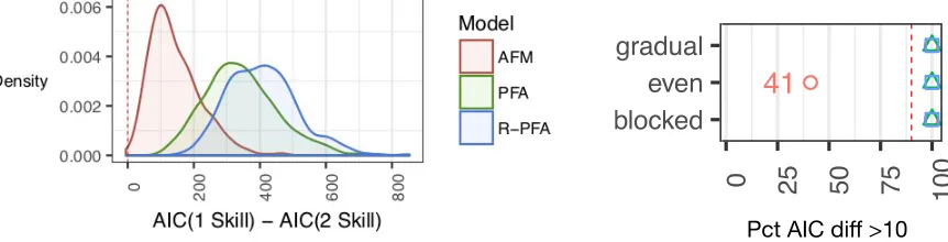
The left side ofFigure 4shows the distributions for the two-skill generative domain model

Algorithm 1isAccurate2Skill: Is a predictive model accurate when two skills are combined?

Require: simConditionsimulation condition_{CurveA, CurveB, InterleavingRegime_}

Require: modelpredictive model

Require: minAICDif minimum AIC difference threshold

dataA_←simulateBKT(simCondition.CurveA)

dataB ←simulateBKT(simCondition.CurveB)

dataT woCurves_←combine(dataA, dataB, simCondition.InterleavingRegime)

f it1_←f itM odel(model, dataT woCurves, Q1)

f it2←f itM odel(model, dataT woCurves, Q2)

(17)

Algorithm 2isAccurate1Skill: is a predictive model accurate when one skill is split?

Require: simConditionsimulation condition{TrueCurve, InterleavingRegime}

Require: modelpredictive model

Require: minAICDif minimum AIC difference threshold

dataOneCurve←simulateBKT(simCondition.T rueCurve)

dataT woCurves_←sample(dataOneCurve, simCondition.InterleavingRegime)

f it1_←f itM odel(model, dataOneCurve, Q1)

f it2←f itM odel(model, dataT woCurves, Q2)

AICDif _←AIC(f it1)₋AIC(f it2)

return minAICDif > AICDif indicates correct model is more accurate.

● ● ●

22

● ● ● ● ● ● ● ● ● ● ● ● ● ● ● ● ● ●

41

● ● ● ● ● ● ● ● ● ● ● ● ● ● ● ● ● ●

26

● ● ● ● ● ● ● ● ● ● ● ● ● ● ● ● ● ● ● ● ● ● ● ● ● ● ● ● ● ● ● ● ● ● ● ● Already Mastered Good High Error Negligible Learning Slow Learning Already Mastered Good High Error Negligible Learning Slow Learning

0 ₂₅ ₅₀ ₇₅

100 0 25 50 75 100 0 25 50 75 100 0 25 50 75 100 0 25 50 75 100

blocked even gradual blocked even gradual blocked even gradual blocked even gradual blocked even gradual

True Split Rate (Pct of AIC differences > 10)

First Cur

ve Shape and Inter

lea

ving Mode

Model

● _AFM

PFA

R−PFA

Second Curve Shape

● ● ●

22

● ● ● ● ● ● ● ● ● ● ● ● ● ● ● ● ● ●

41

● ● ● ● ● ● ● ● ● ● ● ● ● ● ● ● ● ●

26

0 ₂₅ ₅₀ ₇₅

100 0 25 50 75 100 0 25 50 75 100 0 25 50 75 100 0 25 50 75 100

True Split Rate (Pct of AIC differences > 10)

First Cur

ve Shape and Inter

lea

ving Mode

Model

● _AFM

PFA

R−PFA

Second Curve Shape

● ● ●

22

● ● ● ● ● ● ● ● ● ● ● ● ● ● ● ● ● ●

41

● ● ● ● ● ● ● ● ● ● ● ● ● ● ● ● ● ●

26

0 ₂₅ ₅₀ ₇₅

100 0 25 50 75 100 0 25 50 75 100 0 25 50 75 100 0 25 50 75 100

True Split Rate (Pct of AIC differences > 10)

First Cur

ve Shape and Inter

lea

ving Mode

Model

● _AFM

PFA

R−PFA

Second Curve Shape

Pct AIC diﬀ >10

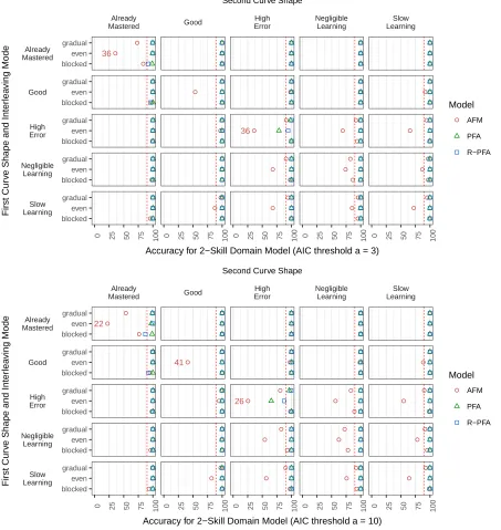
Figure 4: Left: Density of AIC differences for a Good curve Gradually interleaved with another Good curve. Right: Percent of simulations where the two-skill domain model was correctly selected in scenarios where two good curves are interleaved.

when practice on two good skills is interleaved gradually. From this distribution, we can see that AFM, PFA and R-PFA all select the correct two-skill in almost all of the 500 replications. AFM’s margin for AIC differences is smaller than that of PFA and R-PFA, but even AFM’s margin is greater than even the conservative AIC thresholda= 10.

An alternative visualization summarizes the full distribution with respect to a specific AIC difference threshold. The top horizontal line (“gradual”) of the right side ofFigure 4shows the percent of times that each predictive model correctly selected the two-skill model with an AIC threshold of 10. Even though AFM has a much smaller decision margin than PFA or R-PFA, in this gradual interleaving scenario AFM still makes the correct decision almost 100% of the time. However, the middle row indicates that when two good curves are evenly interleaved, AFM correctly selects the two-skill model only 41% of the time.

Using this concise summary visualization, we first discuss the two-skill generative model, and then the one-skill generative model.

4.1. RESULTS FOR THEGENERATIVE MODEL WITHTWO SKILLS

(18)

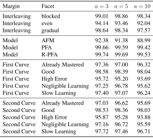
Table 2: Marginal accuracy rates in the two-skill generative model scenarios under different AIC thresholds

Margin Facet a= 3 a= 5 a= 10

Interleaving blocked 99.01 98.86 98.34 Interleaving even 94.14 93.46 92.04 Interleaving gradual 98.64 98.34 97.57

Model AFM 92.38 91.38 88.99

Model PFA 99.66 99.59 99.42

Model R-PFA 99.74 99.69 99.53

First Curve Already Mastered 97.36 97.00 96.32 First Curve Good 98.58 98.39 98.04 First Curve High Error 95.72 95.20 93.69 First Curve Negligible Learning 97.25 96.78 95.62 First Curve Slow Learning 97.40 97.07 96.24 Second Curve Already Mastered 97.03 96.62 95.69 Second Curve Good 98.53 98.36 98.03 Second Curve High Error 95.87 95.28 93.88 Second Curve Negligible Learning 97.16 96.72 95.59 Second Curve Slow Learning 97.72 97.46 96.71

ranging from a drop of0.22%in the marginal performance of R-PFA (froma= 3toa= 10) to a

drop of3.39%in the marginal performance of AFM. Among all the margins, the lowest accuracy

rate is89% for AFM averaged across all simulation scenarios. The three types of interleaving

present grossly similar levels of challenge to the predictive models, ranging from 92.04% to 98.34%. Similarly, the different shapes of the first learning curve or the second learning curve

all lead to accuracy rates of93%or higher.

However, these aggregate results mask important differences among models, among inter-leaving methods, and among curve shapes. To present a more detailed analysis, we collect figures like those in Figure 4 into small multiples in Figure 5 with a = 3 (top) and a = 10

(bottom); results fora = 5are not shown, but similar. This display is essentially a four-way

in-teraction plot, showing the effects of the predictive model (redundantly indicated by point color and shape), the shape of the first curve (Y axis), the shape of the second curve (X axis), and mode of interleaving (subsidiary Y axis in each cell).

For example, the graph from Figure 4 is shown in the second row, second column of on the bottom ofFigure 5. Similarly, the bottom left cell (in both the a = 3 anda = 10figures)

shows that for Slow Learning curves interleaved with Already Mastered curves, all three models have accuracy rates above90%no matter the mode of interleaving. However, for Slow Learning

curves interleaved with other Slow Learning curves (bottom right cell), only PFA and R-PFA have accuracy rates above90%, while AFM only correctly selects the two-skill domain model

(19)

● ● ● 36 ● ● ● ● ● ● ● ● ● ● ● ● ● ● ● ● ● ● ● ● ● ● ● ● ● ● ● ● ● ● ● ● ● ● ● ● 36 ● ● ● ● ● ● ● ● ● ● ● ● ● ● ● ● ● ● ● ● ● ● ● ● ● ● ● ● ● ● ● ● ● ● ● ● Already Mastered Good High Error Negligible Learning Slow Learning Already Mastered Good High Error Negligible Learning Slow Learning

0 ₂₅ ₅₀ ₇₅

100 0 25 50 75 100 0 25 50 75 100 0 25 50 75 100 0 25 50 75 100

Accuracy for 2−Skill Domain Model (AIC threshold a = 3)

First Cur

v

e Shape and Inter

lea ving Mode Model ● AFM PFA R−PFA Second Curve Shape

● ● ● 22 ● ● ● ● ● ● ● ● ● ● ● ● ● ● ● ● ● ● 41 ● ● ● ● ● ● ● ● ● ● ● ● ● ● ● ● ● ● 26 ● ● ● ● ● ● ● ● ● ● ● ● ● ● ● ● ● ● ● ● ● ● ● ● ● ● ● ● ● ● ● ● ● ● ● ● Already Mastered Good High Error Negligible Learning Slow Learning Already Mastered Good High Error Negligible Learning Slow Learning

0 ₂₅ ₅₀ ₇₅

100 0 25 50 75 100 0 25 50 75 100 0 25 50 75 100 0 25 50 75 100

First Cur

v

e Shape and Inter

(20)

MODEL DIFFERENCES The simulations show that the PFA and R-PFA models are generally

very sensitive in teasing apart inappropriately merged skills, and AFM is less sensitive. Under the a = 3 threshold for AIC differences (top figure), R-PFA has an accuracy rate above 90%

in all of the simulation scenarios, and PFA in all but one scenario: High Error curves evenly interleaved with other High Error curves, where it is 79%. When we raise the threshold to

a= 10, the accuracy rate for PFA in this scenario falls further to 65%, and the accuracy rate for

R-PFA falls to 88%. By contrast, AFM often has low accuracy rates, including undera= 3(16

of 75 simulation scenarios) anda= 10(21 scenarios).

INTERLEAVING EFFECTS PFA and R-PFA handle all three interleaving types equally well. However, AFM’s two-skill accuracy rates differ dramatically based on the combination of curve shapes. For example, under the liberal threshold a = 3, for an Already Mastered curve

com-bined with another Already Mastered curve, AFM’s accuracy ranges from 83%under blocked

interleaving to36%when the curves are evenly interleaved (i.e., worse than flipping a coin). At

the conservative thresholda = 10in the same scenario (two Already Mastered curves, evenly

interleaved), AFM only recognized a correct split in22%of the simulations.

For AFM, curves that are interleaved evenly are consistently more difficult to tease apart than gradually interleaved and blocked curves, and this is in large part driving the overall lower performance of AFM. At thea = 3 threshold, AFM struggles to correctly select the two-skill

model with evenly interleaved curves in 12 of 25 curve shape pairs. Under gradual or blocked interleaving with thea = 3threshold, AFM struggles with only 2 pairs of shapes. At a = 10,

AFM has low accuracy rates in 13 of 25 evenly interleaved pairs, 5 gradually interleaved pairs, and 3 blocked pairs.

GENERATING CURVE SHAPE PFA and R-PFA are able to accurately discern a variety of

curve shape pairs. PFA has a relatively low accuracy rate in only one simulation scenario, High Error curves evenly interleaved with other High Error curves. R-PFA is also challenged by the same scenario, but only at the conservative a = 10threshold, and even then, it still correctly

recognizes a split in88%of the simulations.

If we consider the more conservative a = 10 threshold, AFM has more difficulty with the

High Error, Negligible Learning and Slow Learning curves (below 90% in 15/27 scenarios), than with Good and Already mastered (below 90% in 4/12 scenarios).

SHAPE OF COMBINED SINGLE SKILL CURVE Visualization of sample curve shape pairs

(Figure 8, Figure 9, Figure 10in Appendix A) illustrates the challenge of teasing them apart. AFM consistently had lower accuracy rates with Evenly interleaved curves (Figure 9). The curve pairs that challenge AFM the most produce relatively smooth curves when the skills are evenly interleaved. A Slow Learning skill interleaved with an already mastered skill produces a very jagged learning curve in the single-skill coding, and all 3 models chose the correct two-skill model almost 100% of the time, at any threshold. In contrast, when two High Error curves are interleaved, the resulting single-skill coding has a fairly smooth curve, and all 3 models had more difficulty selecting the correct two-skill model. Specifically, AFM preferred the wrong model 74% of the time (a = 10). Other interleaving types can also produce somewhat smooth

(21)

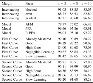
Table 3: Marginal accuracy rates in the two-skill generative model scenarios under different AIC thresholds; 20 students

Margin Facet a= 3 a= 5 a= 10

Model AFM 78.77 75.02 66.47

Model PFA 96.66 95.86 93.91

Model R-PFA 96.03 95.10 92.22

First Curve Already Mastered 92.10 90.89 88.22 First Curve Good 94.29 93.22 90.08 First Curve High Error 84.00 80.68 73.03 First Curve Negligible Learning 90.62 88.84 84.33 First Curve Slow Learning 91.42 89.65 85.34 Second Curve Already Mastered 85.91 83.51 77.00 Second Curve Good 95.11 93.99 90.96 Second Curve High Error 86.56 83.99 78.16 Second Curve Negligible Learning 91.66 90.13 86.62 Second Curve Slow Learning 93.20 91.68 88.28

4.1.1. Sample Size

While the findings above show strong performance by PFA and R-PFA, there must necessarily be limitations to these simple logistic models. A full analysis of these limitations is a substantial project in its own right, but we took a first step: examining the question of how much data is necessary. It is often the case in real data, that some skills are practiced by fewer students than other skills. To model this, we re-ran the simulation with the number of simulated students per skill decreased from 100 to 20. Reducing the sample size highlights some of the differences among predictive models, interleaving modes and curve shapes that were not apparent with a larger sample size (Table 3,Figure 6).

PREDICTIVE MODELS (N=20) AFM accuracy drops with the sample size reduction, with

aggregate accuracy rates ranging from79% (a = 3) to66.47% (a = 10). Ata = 10, AFM’s

accuracy rate remains above90%in only 23 of the 75 simulation scenarios.

PFA and R-PFA remain generally robust to the change in sample size, with aggregate accu-racy rates above92%even ata = 10. However, some curve combinations become challenging

to both models.

In 53 of 75 scenarios, both PFA and R-PFA have accuracy rates of97%or higher; in another

9 scenarios, both models’ accuracy rates are 88% or higher. That leaves 13 scenarios which

these two models find particularly challenging (Table 4), as discussed below.

INTERLEAVING MODES(N=20) Considered at an aggregated level, the interleaving regimes

(22)

(Table 3). The relative order of difficulty is not affected by the reduced sample size: even interleaving is the most difficult, followed by gradual and blocked.

GENERATING CURVE SHAPE (N=20) The same cases which were difficult with 100

stu-dents only become more difficult with 20 stustu-dents, as should be expected. Any combination of High Error, Negligible Learning or Slow Learning is challenging for AFM. Scenarios that have Already Mastered or Good as the second skill, in particular, induce lower accuracy rates than with the higher sample size.

SHAPE OF COMBINED SINGLE SKILL CURVE (N=20) Given how many curve pairs

pre-sented difficulty to AFM, we infer that the 23 scenarios in which AFM could distinguish the two skills must be somehow inherently easier cases. This includes the 12 scenarios where an Already Mastered curve is followed by any other curve shape. This is apparent in the consistently high accuracy rates in the Already Mastered row inFigure 6. Similarly, AFM can often tease apart a Good curve that is Blocked or Gradually interleaved with High Error, Negligible Learning or Slow Learning (Figure 6, row 2). These “inherently easy” scenarios produce a learning curve for the single-skill coding of the domain model that is quite jagged. For example, there’s a dramatic drop in success rate when an Already Mastered curve is blocked with any other curve shape (Figure 8).

In the scenario when two good skills are evenly interleaved, AFM prefers the false one-skill domain model over the correct two-skill model 81% of the time. But when practice is blocked, AFM correctly detects the two skills with accuracy well above 90%, even at this small sample size.

Revisiting a visual example of these curve pairs (Figure 2), it does seem plausible that inter-leaving can cause these differences in accuracy of recognizing a two-skill domain model. Under Blocked interleaving, the single-skill coding produces a learning curve with a dramatic dip in success rate, but in Even interleaving, the single-skill learning curve is relatively smooth. Under Gradual interleaving, this curve pairing may (probabilistically) still have dramatic dips, but the accuracy nonetheless drops, depending on the sample size and AIC threshold.

We turn now to the 13 scenarios in which PFA and R-PFA had accuracy rates less than 88% (Table 4). Any mode of interleaving two High Error curves or two Already Mastered curves is severely challenging for both PFA and R-PFA (6 scenarios). In these scenarios, the single-skill coding produces a relatively smooth learning curve, so that the incorrect single skill model is chosen as more predictive between 20% and 70% of the time, depending on the threshold.

In the condition that the sample size is small and the AIC difference threshold is conservative, there is a pattern of differences between PFA and R-PFA. Specifically, they tend to differ when two curves are blocked, and the population success rates are somewhat close at the end of the first curve and the beginning of the second. For example, when a Good curve is gradually interleaved with an Already Mastered curve, both PFA and R-PFA have accuracy rates near 90%. However, when Good is blocked with an Already Mastered curve, PFA accuracy drops only slightly, whereas R-PFA’s accuracy drops precipitously. There are 7 similar scenarios (bottom section ofTable 4). In each of these 7 scenarios, the learning curve for the single-skill coding has a relatively small dip in the shape of the curve (Figure 8).

(23)

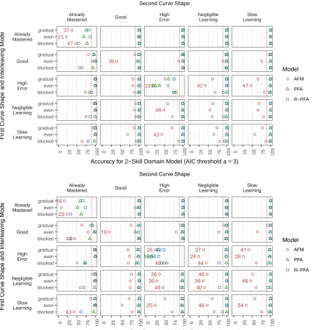
● ● ● 47 21 37 ● ● ● ● ● ● ● ● ● ● ● ● ● ● ● ● ● ● 39 ● ● ● ● ● ● ● ● ● ● ● ● ● ● ● ● ● ● 1936 ● ● ● 48 ● ● ● 43 ● ● ● ● ● ● ● ● ● 42 ● ● ● ● ● ● ● ● ● ● ● ● ● ● ● 47 ● ● ● ● ● ● Already Mastered Good High Error Negligible Learning Slow Learning Already Mastered Good High Error Negligible Learning Slow Learning

0 25 50 75 ₁₀₀ 0 25 50 75 ₁₀₀ 0 25 50 75 ₁₀₀ 0 25 50 75 ₁₀₀ 0 25 50 75 ₁₀₀

First Cur

v

e Shape and Inter

● ● ● 23 16 ● ● ● 44 ● ● ● ● ● ● ● ● ● 43 ● ● ● ● ● ● 19 ● ● ● ● ● ● ● ● ● ● ● ● ● ● ● ● ● ● 48 1634 25 49 ● ● ● 46 30 36 ● ● ● 25 ● ● ● ● ● ● ● ● ● 44 24 37 ● ● ● 40 36 46 ● ● ● 46 ● ● ● ● ● ● ● ● ● 26 41 ● ● ● 46 ● ● ● 34 Already Mastered Good High Error Negligible Learning Slow Learning Already Mastered Good High Error Negligible Learning Slow Learning

0 ₂₅ ₅₀ ₇₅

100 0 25 50 75 100 0 25 50 75 100 0 25 50 75 100 0 25 50 75 100

First Cur

ve Shape and Inter

lea

ving Mode

Model

● AFM PFA

R−PFA

Second Curve Shape

(24)

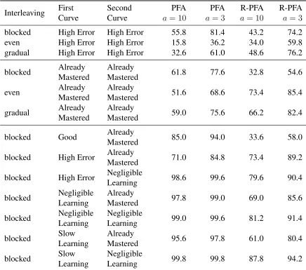
Table 4: Accuracy rates, 20 students, scenarios in which PFA or R-PFA are below 90% accuracy.

Interleaving First_Curve Second_Curve PFA

a= 10

PFA

a= 3

R-PFA

a= 10

R-PFA

a= 3

blocked High Error High Error 55.8 81.4 43.2 74.2 even High Error High Error 15.8 36.2 34.0 59.8 gradual High Error High Error 32.6 61.0 48.6 76.2

blocked Already_Mastered Already_Mastered 61.8 77.6 32.8 54.6

even Already_Mastered Already_Mastered 51.6 68.6 73.4 85.4

gradual Already_Mastered Already_Mastered 59.0 75.6 66.2 82.4

blocked Good Already_Mastered 85.0 94.0 33.6 58.0

blocked High Error Already_Mastered 71.0 84.8 73.4 89.2

blocked High Error Negligible_Learning 98.6 99.6 79.6 90.4

blocked Negligible_Learning Already_Mastered 97.8 99.0 69.0 85.6

blocked Negligible_Learning Negligible_Learning 99.0 99.6 81.2 91.4

blocked Slow_Learning Already_Mastered 95.6 97.8 61.0 80.4

blocked Slow_Learning Negligible_Learning 99.8 99.8 87.8 94.2

of correct attempts in the R-PFA model, and the decay factor applied toR. Given a small sample

of 20 students, there is insufficient data for R-PFA to learn a skill parameter that reflects the dip at the join of the curves. Both PFA and R-PFA improve in accuracy rate at the more liberal AIC thresholda = 3, but more importantly, both models attain very high true accuracy even at

a= 10when the sample size is sufficiently large.

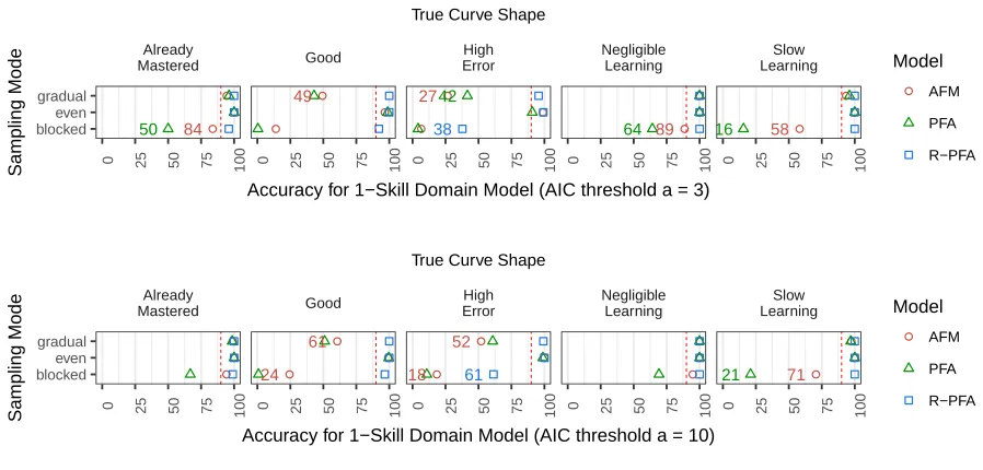
4.2. RESULTS FOR THEGENERATIVE MODEL WITHONE SKILL

In this set of 15 scenarios, we test the accuracy of the predictive models in recognizing the generative (correct) one-skill model rather than an alternative domain model that improperly splits that skill into two skills. This set of scenarios would be analogous to the example where forward and backward computations with simple geometric figures were proposed to be two skills, but found to be a single skill (Koedinger et al., 2012).

(25)

a = 10. In this set of scenarios, as the AIC difference threshold increases, the models become

more likely to choose the one-skill model, because the two-skill model must meet the higher, more conservative, threshold to be considered a better model. There are substantial differences across all facets: predictive models, modes of interleaving, and true curve shapes.

The small-multiples plot (Figure 7) shows the accuracy rate (x-axis) across the three-way interaction of true curve shape (secondary x-axis), interleaving mode (y-axis), and the predictive model (point color and shape). At either threshold, and in all facets of the interaction, R-PFA is consistently the most accurate model for the single-skill model. PFA and AFM vie for second place, depending on the interaction.

PREDICTIVE MODELS On average, AFM and PFA have mediocre performance, with the

highest aggregate accuracy rates at 81% and72%, respectively. Both models struggle in all 5

blocked scenarios, though there is an interaction discussed below. On true Negligible Learning curves, performance is borderline (AFM has an accuracy of 89% witha = 3); however, in the

High Error and Good cases, AFM prefers the incorrect two-skill coding in more than 75% of replications.

R-PFA performs well, with an aggregate accuracy rate above 95%for all thresholds. When

the generative curve is Already Mastered, Negligible Learning or Slow Learning, R-PFA has almost-perfect accuracy rates across all interleaving modes. For Good curves, the accuracy is still above 90%. R-PFA struggles in one case, namely where a High Error curve is falsely split into two curves using blocked interleaving.

INTERLEAVING There are strong effects of interleaving regime. When the one-skill curve is

split using even interleaving, the predictive models are generally accurate at recognizing the one-skill model (accuracy above 82%). Accuracy decreases under gradual interleaving (above 82%), and under blocked interleaving, accuracy is little better than a coin flip (between 54% and 62%). This is the opposite of the two-skill generative model, where accuracy is lowest with even interleaving and higher with gradual or blocked interleaving.

GENERATING CURVE SHAPE The generative curve shape affects the accuracy rate

dramati-cally. The Already Mastered and Negligible Learning generative curves can be recognized with high accuracy (above 91% and 95%, respectively). These two curves are similar to straight lines with relatively flat slopes, and have the least curvature out of all 5 curve types; and no matter the interleaving regime, the two-skill coding produces learning curves that are parallel, if not almost identical (Figure 3). Thus, it makes sense that a predictive model could easily recognize the one-skill model.

(26)

Table 5: Marginal accuracy rates for the one-skill generative model under different AIC thresh-olds

Margin Facet a = 3 a= 5 a= 10

Model AFM 73.99 76.01 80.71

Model PFA 66.72 68.29 71.63

Model R-PFA 94.72 95.51 97.08

True Curve Already Mastered 91.16 92.51 95.29 True Curve Good 66.04 67.11 70.24 True Curve High Error 55.69 59.13 66.82 True Curve Negligible Learning 94.71 95.13 96.00 True Curve Slow Learning 84.78 85.80 87.33

● ● ● 84 50 ● ● ● 49 ● ● ● 38 2742 ● ● ● 89 64 ● ● ● 58 16 Already Mastered Good High Error Negligible Learning Slow Learning

0 25 50 75 ₁₀₀ 0 25 50 75 ₁₀₀ 0 25 50 75 ₁₀₀ 0 25 50 75 ₁₀₀ 0 25 50 75 ₁₀₀

Sampling Mode

Model

● AFM

PFA

R−PFA True Curve Shape

● ● ● ● ● ● 24 61 ● ● ● 18 61 52 ● ● ● ● ● ● 71 21 Already Mastered Good High Error Negligible Learning Slow Learning

0 ₂₅ ₅₀ ₇₅

100 0 25 50 75 100 0 25 50 75 100 0 25 50 75 100 0 25 50 75 100

Sampling Mode

Model