https://doi.org/10.5194/essd-11-341-2019 © Author(s) 2019. This work is distributed under the Creative Commons Attribution 4.0 License.
Atmospheric data set from the Geodetic Observatory
Wettzell during the CONT-17 VLBI campaign
Thomas Klügel, Armin Böer, Torben Schüler, and Walter Schwarz
Federal Agency for Cartography and Geodesy, Geodetic Observatory Wettzell, 93444 Bad Kötzting, Germany
Correspondence:Thomas Klügel (thomas.kluegel@bkg.bund.de)
Received: 23 October 2018 – Discussion started: 16 November 2018 Revised: 16 January 2019 – Accepted: 7 February 2019 – Published: 28 February 2019
Abstract. Continuous very long baseline interferometry (VLBI) observations are designed to obtain highly ac-curate data for detailed studies of high-frequency Earth rotation variations, reference frame stability, and daily to sub-daily site motions. During the CONT-17 campaign that covered a time span of 15 days between 28 Novem-ber and 12 DecemNovem-ber 2017, a comprehensive data set of atmospheric observations was acquired at the Geodetic Observatory Wettzell, where three radio telescopes contributed to three different networks which have been es-tablished for this campaign. These data were supplemented by weather model data. The data set is made available to all interested users in order to provide an optimal database for the analysis and interpretation of the CONT-17 VLBI data. In addition, it is an outstanding data set for the validation and comparison of tropospheric param-eters resulting from different space techniques with regard to the establishment of a common atmosphere at co-location sites.
The regularly recorded atmospheric parameters comprise many meteorological quantities (pressure, tempera-ture, humidity, wind, radiation, and precipitation) taken from the local weather station close to the surface, solar radiation intensity, temperatures up to 1000 m above the surface from a temperature profiler, total vapor and liquid water content from a water vapor radiometer, and cloud coverage and cloud temperatures from a nubis-cope. Additionally, vertical profiles of pressure, temperature, and humidity from radiosonde balloons and from numerical weather models were used for comparison and validation.
The graphical representation and comparison show a good correlation in general but also some disagreements in certain weather situations. While the accuracy and the temporal and spatial resolution of the individual data sets are very different, the data as a whole characterize the atmospheric conditions around Wettzell during the CONT-17 campaign comprehensively and represent a sound basis for further investigations (https://doi.org/10. 1594/PANGAEA.895518; Klügel et al., 2018).
1 Introduction
1.1 Geodetic VLBI observations and CONT continuous measurement campaigns
The International VLBI (Very Long Baseline Interferome-try) Service for Geodesy and Astrometry (IVS) coordinates geodetic VLBI observing programs (Nothnagel et al., 2017). VLBI is important since it is the only geodetic technique ca-pable of deriving the full set of Earth orientation parame-ters. The IVS has organized special measurement campaigns called “CONT” approximately every 3 years since 2002.
Figure 1.The Geodetic Observatory Wettzell, with atmospheric sensors highlighted in blue.
1.2 The Geodetic Observatory Wettzell and the purpose of atmospheric observations
The Geodetic Observatory Wettzell (GOW) features two SLR (Satellite Laser Ranging) telescopes, several GNSS (Global Navigation Satellite System) reference stations, and a DORIS (Doppler Orbitography and Ranging Integrated by Satellite) beacon, as well as three VLBI telescopes (Schüler et al., 2015). All three radio telescopes participated in CONT17, each of them in one of the three different net-works. VLBI, GNSS, and DORIS all operate in the mi-crowave frequency domain. In this case, the atmosphere is a major complicating factor reducing the accuracy (Petit and Luzum, 2010). Consequently, the set of atmosphere sensors at the Geodetic Observatory Wettzell has been substantially enhanced in recent years to provide means to better deal with this problem. The propagation delays induced by the iono-sphere can be compensated for with the help of measure-ments taken at at least two different frequencies.
However, the troposphere (and to a lesser extent also the stratosphere) remains a problem. The microwave signals are delayed when passing through these layers, and these effects
Table 1.Sensors of the local weather station. Except for the pressure sensor, the height is given in meters above the surface. Specified accuracies are manufacturer information.
Measured Wind Wind Air temperature Relative humidity Soil Air pressure Precipitation
quantity: direction speed moisture
Sensor ID: WD WS T1 T2 RH1 RH2 SM P R1 R2
Height: 10 m 10 m 10 m 7 m 10 m 7 m −0.5 m 609.3 m a.s.l. 1 m 1 m Type: Lambrecht Lambrecht Lambrecht TRIME-EZ Paroscientific Thies
Nieder-14512 G3 809 MU 809 MU 740–16B schlagsgeber
Measuring 0– 0– −30–70◦C 5 % RH–100 % RH 0 %–95 % 800–1100 hPa (0.1 mm resolution) range: 360◦ 35 m s−1
Accuracy: 1 % 2 % 0.1◦C uncertainty at 0◦C 2.5 % RH 2 % SM 0.1 hPa, stable 10 % of reading
of range of range <0.1 hPa yr−1
2 Study area and instrumentation
The Geodetic Observatory Wettzell is located in eastern Bavaria on a flat mountain ridge about 600 m a.s.l., that is, above standard elevation zero (NHN) of the German height system (DHHN). The topography in the surroundings ranges from valley floors (∼400 m a.s.l.) to mountain ridges (∼1000 m a.s.l.). Land coverage is characterized by grass-land and forest. A plan view of the observatory with the in-strument locations is depicted in Fig. 1. The following sec-tions give a description of the instruments deployed and the quantities measured.
2.1 Local weather station
The temperature, humidity, and wind sensors of the local weather station are mounted on a concrete tower at 7 and 10 m height above the surface (Table 1). The air pressure sen-sor is inside the 20 m radio telescope control building, and the rain gauges are mounted on a platform as shown in Fig. 1. Data are continuously acquired, and averages are recorded once per minute. For wind direction and wind speed, mini-mum and maximini-mum values measured within 1 min are also stored, indicated by “<” and “>”. The heated rain gauges measure snow as well and record the sum over 1 min.
2.2 Radiation sensor
As an addition to the meteorological station, global radiation is measured using a pyranometer, Thies CM 11. At the same place a net radiometer (Kipp & Zonen NR Lite) measures the difference between radiation from above, i.e., the sun and the sky, and from below, i.e., the soil surface. Both sensors are installed 1.5 m above the grass surface. The sampling rate is 10 min.
2.3 Temperature profiler
A quasi-continuous record of temperatures in the atmosphere up to 1000 m height is realized by a radio wave radiometer, MTP-5, from R.P.O. Attex. The microwave receiver mea-sures the blackbody thermal radiation of the atmosphere at a frequency of 56.6 GHz. The intensity of the radiation is a function of the temperature. By scanning the atmosphere at different elevation angles, the operating software computes temperatures at different heights in 50 m steps up to 1000 m, under the assumption of a horizontal temperature layering. The basic principle and some field examples are described in Peña et al. (2013).
The temperature profiler is installed on a tower at 619 m a.s.l. and 10 m above ground. A complete profile is recorded every 5 min. The measurement uncertainty in-creases with height and is specified to be 0.2 to 1.2◦C, de-pending on the profile type and height.
2.4 Water vapor radiometer
On the same tower as the temperature profiler, a water va-por radiometer, Radiometrics WVR-1100, is installed. It is a microwave receiver measuring the intensity of atmospheric radiation at 23.8 and 31.4 GHz. The water vapor dominates the 23.8 GHz observations, whereas the cloud liquid in the atmosphere dominates the power in the 31.4 GHz channel. This allows the simultaneous determination of integrated wa-ter vapor and liquid wawa-ter along the line of sight. From the measured brightness temperatures at both frequencies, Tb23 and Tb31, the frequency-dependent atmospheric opacitiesτ23 andτ31are calculated. The water vapor and liquid water con-tent and the path delay are obtained using the following rela-tionships:
Table 2.Retrieval coefficients used (in centimeters).
c0vap c1vap c2vap c0liq c1liq c2liq c0del c1del c2del
0.0045 23.1680 −13.9475 −0.0022 −0.2705 0.5853 0.0678 151.4489 −89.7247
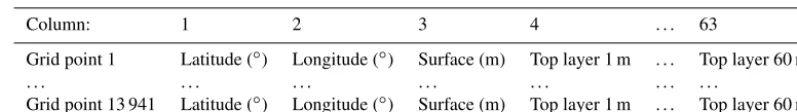
Table 3.Structure of the grid file “we_iconeu_4deg.grd”.
Column: 1 2 3 4 . . . 63
Grid point 1 Latitude (◦) Longitude (◦) Surface (m) Top layer 1 m . . . Top layer 60 m
. . . .
Grid point 13 941 Latitude (◦) Longitude (◦) Surface (m) Top layer 1 m . . . Top layer 60 m
The retrieval coefficientsc0,c1, andc2 are site-dependent and have to be determined from a history of radiosonde ob-servations from a representative site. The retrieval coeffi-cients used in this work are valid for Munich and displayed in Table 2. The blackbody temperature, TkBB, as given in col. 4 of the data file, is only used to establish the tempera-ture coefficient of the instrument gain. A description of the determination of atmospheric water vapor using microwave radiometry is given, e.g., in Elgered et al. (1982).
The instrument performs about one measurement per minute in one particular direction. In azimuth steps of 30◦, elevation scans between 20◦ and 160◦ are carried out; i.e., the scan passes over the zenith direction. For a complete scan of the entire sky, it takes about 90 min. In order to obtain the zenith delay only, all lines with 90◦elevation have to be ex-tracted from the data files. This results in 198 zenith data points per day.
The accuracy of the brightness temperature measurement is specified with 0.5 K. The accuracy of the resulting water vapor and liquid water contents and phase delays strongly depends on the instrument calibration, i.e., the retrieval coef-ficients used.
2.5 Cloud detector
The cloud detector or nubiscope measures the thermal radi-ation of the sky in one particular direction. Since clouds ab-sorb radiation from the sun and reflected infrared radiation from the ground, the temperature of the cloud base is sig-nificantly higher than the clear sky. By scanning the entire sky, a map of the cloud coverage can be generated. As low clouds generally yield higher temperatures than high clouds, additional information regarding the height of the clouds is obtained. Taking into account the horizon effect, that is, the temperature increase from zenith to horizon, the processing software determines the fraction of low-, medium- and high-level clouds, the coverage, temperature, and height of the main cloud base, and the temperature and height of the lowest clouds. Further information is given on the manufacturer’s website (Sattler, no year).
The cloud detector is installed on an observation plat-form on the roof of the Twin Telescope operation building at 625 m a.s.l. and 9 m above the surface. The recorded heights of the cloud base refer to the instrument height. A complete scan of the sky is done once every 10 min.
2.6 Radiosondes
Every day during the CONT17 experiment, radiosonde bal-loons were launched at 8:00 and 14:00 UTC at the launch site depicted in Fig. 1. We used Graw DFM-09 radiosondes and helium-filled Totex 350 balloons with 300 g buoyancy. The transmission rate is one data set per second. The radiosondes are equipped with a GPS receiver, permitting an absolute lo-calization with an accuracy of 5 m in horizontal and 10 m in vertical position. The tracking allows precise measurements of wind speed and wind direction at different heights, with an accuracy of 0.2 m s−1, and ascent and descent rates. The air pressure is computed from the surface pressure at the station, the geopotential height, and the temperature, with an accu-racy of 0.3 hPa. The accuaccu-racy of the temperature and relative humidity sensors is specified with 0.2◦C and 4 %, respec-tively. The relative humidityhrel can be expressed as water vapor pressureeusing
e=es·
hrel
100 (4)
and the Magnus formula according to Sonntag (1990) for the saturation vapor pressure for water in hPa
es=6.112·e
17.62·T
243.12+T, (5)
with the temperatureT in◦C.
Table 4.Parameters from linear regression between temperatures from radiosonde ascents (x) and temperature profiler (y): slopeb,
yaxis offseta, rms fit error, and rms of temperature differences.
Height b a rms rms
(m) (◦C) error difference (◦C) (◦C)
0 0.825 −0.215 1.128 1.488 50 0.833 0.362 1.065 1.342 100 0.866 0.468 0.843 1.126 150 0.902 0.419 0.720 0.942 200 0.932 0.518 0.587 0.857 250 0.933 0.434 0.592 0.821 300 0.927 0.410 0.636 0.869 350 0.927 0.274 0.761 0.912 400 0.928 0.277 0.823 0.975 450 0.934 0.179 0.865 0.970 500 0.932 0.121 0.913 1.009 550 0.930 0.101 0.997 1.089 600 0.932 0.193 1.083 1.197 650 0.932 0.303 1.160 1.308 700 0.935 0.545 1.238 1.483 750 0.932 0.679 1.280 1.607 800 0.931 0.898 1.248 1.734 850 0.927 0.975 1.233 1.800 900 0.921 1.137 1.235 1.959 950 0.913 1.173 1.229 2.033 1000 0.907 1.270 1.193 2.141
3 Weather models
3.1 DWD ICON-EU model
For the time span covering the CONT17 campaign, a data set was extracted from the ICON-EU model from the Ger-man Weather Service (Deutscher Wetterdienst, DWD) con-taining pressure, temperature, and humidity data at different height levels. The ICON-EU model is a refined domain (lo-cal nest) of the global ICON (ICOsahedral Nonhydrostatic) model, whose grid is made up by a set of nearly equal spher-ical triangles spanning the entire Earth (Reinert et al., 2018). The ICON-EU nest is refined by dividing each triangle into four subtriangles, resulting in a grid spacing of ∼6.5 km. It includes 60 height levels up to 22.5 km. The physical pa-rameters at the top of the model are controlled by the global model reaching a height of 75 km.
The extracted subset covers a radius of 4◦ (∼445 km) around the GOW. The structure of the grid file “we_iconeu_4deg.grd” is given in Table 3, where each line represents one of the 13 941 grid points. The data files are named “we_iconeu_4deg_yyyymmddhh.xxx”, where yyyy denotes the year, mm the month, dd the day, hh the hour, and xxx the physical quantity.
– pre: air pressure (hPa)
– tem: temperature (K)
– hum: water vapor pressure (hPa)
As the model is built up of 60 layers, the temperature and humidity files comprise 60 columns and the pressure file 61 columns, since temperature and humidity are given within the layers and the pressure at the layer boundaries. Each line represents the same grid point as given in the grid file.
The model data represent the atmospheric analysis fields at the beginning of each forecast run and are computed every 3 h using assimilated observed data.
3.2 NCEP model
As a comparative data set, both zenith hydrostatic and wet delays (ZHDs and ZWDs) from the NCEP (National Cen-ter for Environmental Prediction) global numerical weather model are provided. This data set is derived from GDAS (Global Data Assimilation System) and GSF (Global Fore-casting System) weather fields. The derivation of these tro-pospheric path delay data requires some explanation because only one dimensional output file from the GDAS numeri-cal weather model (so-numeri-called “surfaces fluxes”) was used. From our experience, zenith total delays are expected to re-veal a standard deviation approaching 1 cm for the region of Wettzell. This is slightly less accurate than the estimation of tropospheric delays using GNSS permanent stations (see Fig. 9) but still useful for a number of applications.
The original weather model output data can be found on the ftp server at http://ftp.ncep.noaa.gov/ (last access: 22 February 2019) in the directory “/data/nccf/com/gfs/prod”, all available in standard grib2 format. Note that this is a rolling real-time archive. Regions of interest are routinely extracted at our observatory and converted into a tailored format, addressing the specific needs of space geodesy. Analysis fields are used whenever possible (every 6 h) with one 3 h prediction in between.
The necessary information is horizontally interpolated and vertically reduced to the central GNSS station WTZR at the observatory. The horizontal interpolation approach is de-picted in Schüler (2001, p. 197ff) using the four nearest neighbors, but as a modification, bilinear functions of type
a0+a1·φ+a2·λ+a3·φ·λare employed for interpolation of the surface flux data, wherea0, ... ,3are the interpolation coef-ficients determined from the four nearest neighbors,φis the latitude of the interpolation site, andλis its longitude. Verti-cal reduction to the target height is important. The TropGrid2 model (Schüler, 2014) is used for this purpose. TropGrid2 is a global gridded 1◦×1◦ model containing reduction coef-ficients for all quantities needed. The coefcoef-ficients of these reduction functions were derived using 9 years of numerical weather model data.
Figure 2.Traces of radiosonde balloons, with maximum heights indicated by red stars.
(Saastamoinen, 1972):
ZHD= 0.0022767·p
1−0.00266·cos(2φ)−0.00028·h, (6)
with the pressure p (hPa), the ellipsoidal height h (km), and the geographic latitude φ of the station. The deriva-tion of ZWD (zenith wet delay) requires more effort, but GDAS/GSF surface fluxes are a very attractive resource since these weather fields already contain the total col-umn atmospheric water vapor (IWV, integrated water vapor). These values are converted into ZWD with knowledge of
the weighted mean temperature of the atmosphereTM (see Schüler, 2001, p. 184ff).TMitself is substituted in the stan-dard product by a surface temperature conversion function available on the TropGrid2 data grid. After conversion, ZWD is vertically reduced and horizontally interpolated to the tar-get height.
4 Data availability
All data sets are available at
Figure 3.Height–distance plot of all balloon ascents. The height axis is exaggerated by a factor of 2.
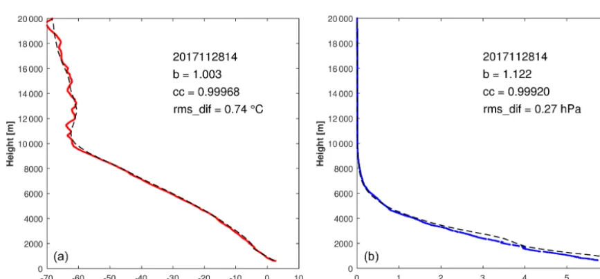
Figure 4.Height profiles of temperature(a)and water vapor content(b)of one particular radiosonde ascent as compared to the weather model profile at the launch location (dotted line). The correlation parameters between both series (b: slope of the best fit line, cc: correlation coefficient, rms_dif: rms of differences) are indicated.
al., 2018). In all time series, the first column represents UTC date and time, with the format yyyy-mm-ddThh:mm:ss. The columns are separated by tabs (\t) in all files with the exception of the ICON-EU model data for which blanks (\s) are used. The ICON-EU model data are stored in a compressed tar archive; all other files are available as ASCII text files. The file description is given in Table 5.
5 Data representation and results
The data from the radiosonde balloon ascents give a direct temperature and humidity profile through the troposphere and are thus a proper tool to validate the weather model and to calibrate radiation-based sensors like the water vapor ra-diometer or the temperature profiler. The radiosonde ascents
between 28 November and 15 December reached heights be-tween 5.6 km (14 December 2017 08:00 launch) and 25.8 km (13 December 2017 08:00 launch) with an average at 19 km. The average ascent rates were between 4 and 6 m s−1in most cases. The maximum covered horizontal distance to the burst point was 170 km towards northeast (Fig. 2). The horizontal drift is 2–8 km per kilometer of height in most cases (Fig. 3). This means that the tropospheric data up to 10 km height are representative of a region 20–80 km mainly to the east of the launch site.
tem-Figure 5. Temperature profiler (T-profiler) time series at particular heights compared to the temperature record of weather station and radiosonde data at equivalent heights (dots).
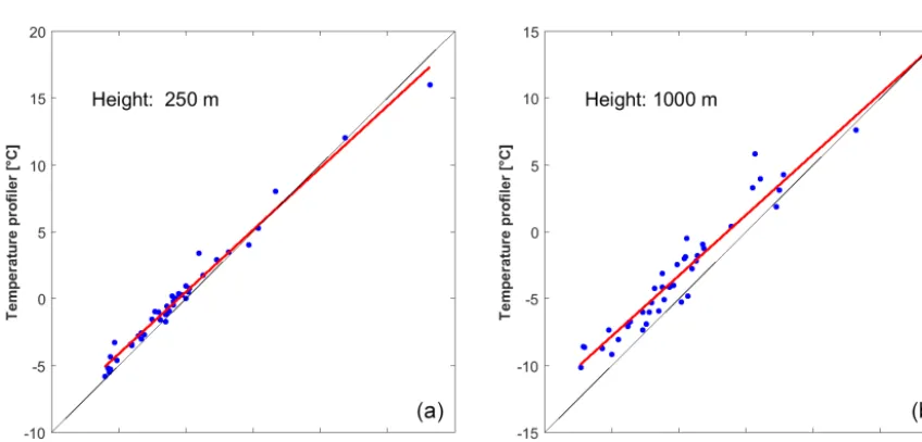
Figure 6.Linear regression between temperatures from radiosonde ascents and contemporaneous profiler records at two particular heights. For regression parameters, see Table 4.
peratures and those from the radiosondes interpolated to the model layer heights yields linear trends (b) and Pearson cor-relation coefficient (cc) values very close to 1, underlining the high consistency of the model. The only misfit occurred at the 1 December 2017 08:00 launch. In this particular case the measured height seemed to be corrupted. Ignoring this launch, a mean correlation coefficient of 0.9992 is obtained.
Figure 7.Integrated water vapor (IWV) content as measured by the water vapor radiometer (WVR) compared to IWV values derived from weather model and radiosonde data. WVR spikes coincide with periods of rain.
Figure 8.Linear regression between integrated water vapor (IWV) content derived from radiosonde data and that from water vapor ra-diometer (WVR) and weather model data. The two outliers were removed in the regression.
and 1.2 in most cases. The mean correlation coefficient is 0.9898.
A graphical representation of measured pressure, temper-ature, and water vapor profiles from all radiosonde ascents in
comparison to model data is given in the Supplement of the data repository.
The radiosonde data can also be used to validate the tem-perature profiler. Figure 5 shows the traces of the temtem-perature profiler at six different height levels compared to tempera-tures measured by the radiosondes at the equivalent height. While a good coincidence is given at heights up to 400 m, the higher levels yield systematically higher temperatures using the profiler. The root mean square (rms) of the temperature differences at a particular height increases from 0.82 at 250 m up to 2.14 at 1000 m (Table 4). This behavior is underlined by the parameters of linear regression between both temper-atures. The slope of the regression line (b) is always lower than 1, and theyaxis offset (a) increases with height. This in-dicates that the profiler particularly underestimates the lower temperatures at higher levels. Examples of one better and one worse agreement are given in Fig. 6.
One quantity inferred from the measured sky brightness temperatures by the water vapor radiometer is the integrated water vapor content given in height of the equivalent wa-ter column. In order to compare this quantity with weather model and radiosonde data, the water vapor pressureewas converted to specific humiditysusing the following relation-ship (e.g., Simmer, 2006):
s= 0.622·e
p−0.378·e. (7)
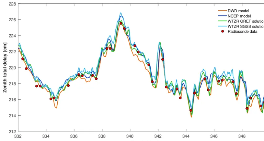
Figure 9.Zenith total delays (ZTDs) derived from numerical weather models, GNSS solutions, and radiosonde data.
Figure 10.Linear regression between zenith total delays (ZTDs) derived from radiosonde data and those derived from numerical weather models and GNSS solutions.
general agreement is good; however, the WVR produces out-liers during periods of rain. This known issue is a conse-quence of rain droplets resting on the radiometer window and falsifying the results, even after the rainfall stopped. This can clearly be seen in Fig. 7 at the beginning of day 345, when after the end of the rain the WVR still yields anoma-lous high IWV values. The linear regression with radiosonde
data shows a fairly good agreement of both the WVR and the weather model when the outliers are removed (Fig. 8). If not, the WVR tends to slightly overestimate the water va-por content. The two outliers in the WVR data are due to raindrops after rainfall on day 338 (afternoon) and day 345 (morning) and removed in the computation of the regres-sion parameters. It should be noted, however, that the re-trieval coefficients used here are valid for Munich, which is 200 km away, since a reliable determination of retrieval co-efficients requires continuous radiosonde data over at least 1 year, which were not available at our site. Thus the total ac-curacy of the estimated water vapor and liquid water content, for which uncertainties from the brightness temperature mea-surement and retrieval coefficients add up, cannot be speci-fied. In addition, the vertical profile of the radiosonde is not necessarily representative of the launch site due to the hori-zontal drift of the balloon (see Fig. 3).
The water content is an important quantity for the estima-tion of the zenith total delay (ZTD), which is the delay radio waves undergo during their propagation through the atmo-sphere. The zenith delays can be mapped to the slant path using geometric relationships, e.g., the Niell mapping func-tion (Niell, 1996) or the Vienna mapping funcfunc-tion (Böhm et al., 2006). The ZTD can be split into a dry, hydrostatic part (zenith hydrostatic delay, ZHD) and a wet part (zenith wet delay, ZWD). Both zenith delay components are obtained through vertical integration of the refractivity indicesNhyd andNwet for each model layer over the entire model. The hydrostatic refractivity indexNhyd only depends on the air densityρ:
Table 5.Description of the data set.
Data set File Content
Meteorological observations
CONT-17_Wettzell_meteo.tab See Table 1.
Global and net radiation
CONT-17_Wettzell_rad.tab Shortwave downward (global) radiation and net radiation (W m−2).
Temperature profile CONT-17_Wettzell_Tpro.tab Radiometric temperatures (◦C) between 0 and 1000 m above the ground, ambient temperature in the last column.
Water vapor and liquid water content
CONT-17_Wettzell_vapo.txt Water vapor radiometer data: Tb23, Tb31: brightness tempera-tures (K), TkBB: blackbody temperature (K), VapCM, LiqCM: in-tegrated water vapor and liquid water content (cm water column), DelCM: radiometric delay (cm), AZ, EL: azimuth and elevation (◦), Tau23, Tau31: atmospheric opacities,T_amb: ambient tem-perature (◦C), RH: relative humidity (%),P: pressure (hPa), rain: rain identifier (arbitrary units).
Cloud coverage and cloud temperatures
CONT-17_Wettzell_nubi.txt Pr: precipitation flag, Tgrnd: ground temperature (◦C), Tbase: model base temperature (◦C), Tzero: air temperature (◦C), Tblue: infrared temperature of clear sky at zenith (◦C), type (clear sky, cirrus only, broken clouds, overcast, transparent clouds, low trans-parent clouds, fog, reduced visibility), ClCov: total cloud cover-age (%),<MCB: clouds below main cloud base (%), MCB: cov-erage (%), base temperature (◦C), and height (m) of main cloud base, LLC: coverage of low-level clouds (%), MLC: coverage of medium-level clouds (%), HLC: coverage of high-level clouds (%), lowestCl: base temperature (◦C) and height (m) of lowest clouds.
Radiosonde data CONT-17_Wettzell_radios.tab Sonde ID, time (s after launch), latitude (◦), longitude (◦), altitude (m), pressure (hPa), temperature (◦C), relative humidity (%), wind speed (m s−1), wind direction (◦clockwise from north), geopoten-tial height (m).
ICON-EU model data iconeu_wtz.grd Latitude (◦), longitude (◦), and height levels (m) (see Table 3) iconeu_wtz_yyyymmddhh.pre Air pressure (hPa) at layer boundaries (see Sect. 3.1) iconeu_wtz_yyyymmddhh.tem Temperature (K) within layers (see Sect. 3.1)
iconeu_wtz_yyyymmddhh.hum Water vapor pressure (hPa) within layers (see Sect. 3.1)
NCEP model data and zenith path delays
CONT-17_Wettzell_ncep-sflux-zpd.tab Surface fluxes from NCEP model and derived zenith path de-lays (see Sect. 3.2) interpolated to WTZR location: air pressure (hPa), temperature (◦C), relative humidity (%), zonal and merid-ional wind speed (m s−1), cloud coverage (%), precipitation rate (mm h−1), weighted mean temperature (◦C), zenith total delay (ZTD; mm), zenith hydrostatic delay (ZHD; mm), and zenith wet delay (ZWD; mm) with standard deviations.
Zenith path delays from GNSS analysis
CONT-17_Wettzell_zpd_sgss_gref.tab ZTD (mm) from local network analysis using SGSS software with 68 % confidence interval C of median value, ZTD (mm) from GREF analysis with standard deviations.
with the hydrostatic refraction constant k1=77.6 K hPa−1 and the specific gas constant for dry air Rd= 287.05 J kg−1K−1. The density follows the equation of state for ideal gases:
ρ= p
Rd·Tv
, (9)
with the pressurep and the virtual temperature Tv in each layer.Tv is the equivalent temperature of dry air with the same density as wet air and is computed from the air tem-peratureT and the specific humidity s according to Emeis (2000):
Figure 11. Total cloud coverage (dark blue) and portion of medium- plus high-level clouds (light blue) in comparison with the global radiation as measured by the pyranometer.
The wet refractivity indexNwetis a function of the partial water vapor pressureeand the temperatureT in kelvin:
Nwet=k20·
e T +k3·
e
T2, (11)
with the refraction constants k02=22.1 K hPa−1 and k3= 370 100 K2hPa−1 (Bevis et al., 1994). The compressibility factor accounting for non-ideal gas behavior is neglected in this case.
For the vertical integration, the refractive index at each layer multiplied by the layer thickness is summed over all model layers. Above the upper boundary of the ICON-EU model at 22.5 km height, the remaining part of ZHD, being on the order of 7–8 cm, is computed according to Eq. (6), with the pressure and height taken at the top of the model instead of the surface. The contribution of the atmosphere above 22.5 km to the ZWD can be neglected since the wa-ter vapor content is close to zero. A similar procedure was applied to determine the zenith delays ZHD and ZWD from radiosonde data.
The total delays ZTD, the sum of ZHD and ZWD as com-puted from weather model and radiosonde data, are displayed in Fig. 9 and compared to the ZTD estimation from GNSS analyses. One solution is taken from the BKG GNSS Data Center, a routine analysis of station WTZR as part of the of the GREF network (https://igs.bkg.bund.de/dataandproducts/ browse, last access: 22 February 2019) using Bernese 5.2 software; the other solution is derived from the Wettzell lo-cal array using the in-house analysis software SGSS. The re-ported values represent the mean and the 68 % confidence interval of the eight Wettzell GNSS stations each being an-alyzed in three different regional networks. The confidence intervals give a more realistic error estimation and are thus larger than the standard deviations of a single analysis given in the GREF data.
A time series of the different ZTD values is displayed in Fig. 10. All traces show a similar behavior. The GNSS anal-yses reveal more details as a consequence of the higher sam-pling rate of 1 h. Taking the radiosonde data as a reference, the DWD model tends towards lower (2–3 mm) ZTD values and the NCEP model towards higher (5–6 mm) ZTD values. The best coincidence with the radiosonde-derived ZTD gives the GNSS solutions with correlation coefficients up to 0.992. The cloud coverage as recorded by the nubiscope and the global radiation as measured by the pyranometer are dis-played in Fig. 11.
Supplement. The supplement related to this article is available online at: https://doi.org/10.5194/essd-11-341-2019-supplement.
Author contributions. TS initiated the project and the radiosonde balloon ascents, which were performed under supervision of WS. AB and WS maintained the instruments and provided the measured data. Model data were prepared by TS and TK. TK compiled the data and prepared the manuscript with contributions from all co-authors.
Competing interests. The authors declare that they have no con-flict of interest.
Acknowledgements. The support from the entire team of the Geodetic Observatory Wettzell is gratefully acknowledged.
Edited by: Kirsten Elger
References
Behrend, D.: Successful Start of CONT17, IVS Newsletter, 49, 1, available at: https://ivscc.gsfc.nasa.gov/publications/newsletter/ issue49.pdf (last access: 22 February 2019), 2017.
Behrend, D., Thomas, C., Gipson, J., and Himwich, E.: Planning of the Continuous VLBI Campaign 2017 (CONT17), in: Pro-ceedings of the 23rd European VLBI Group for Geodesy and Astrometry Working Meeting, edited by: Haas, R. and Elgered, G., Gothenburg, Sweden, 142–145, available at: http://www.oso. chalmers.se/evga/23_EVGA_2017_Gothenburg.pdf (last access: 22 February 2019), 2017.
Bevis, M., Businger, S., Chiswell, S., Herring, T., Anthes, R., Rocken, C., and Ware, R.: GPS Meteorology: Map-ping Zenith Wet Delays onto Precipitable Water, J. Appl. Meteorol., 33, 379–386, https://doi.org/10.1175/1520-0450(1994)033<0379:GMMZWD>2.0.CO;2, 1994.
Böhm, J., Werl, B., and Schuh, H.: Troposphere mapping functions for GPS and Very Long Baseline Interferometry from European Centre for Medium-Range Weather Forecasts operational analysis data, J. Geophys. Res., 111, B02406, https://doi.org/10.1029/2005JB003629, 2006.
Elgered, G., Rönnäng, B. O., and Askne, J. I. H.: Measurements of atmospheric water vapour with microwave radiometry, Radio Sci., 17, 1258–1264, AGU, 1982.
Emeis, S.: Hirt’s Stichwörterbücher: Meteorologie in Stichworten, ISBN 3-443-03108-0, Borntraeger, Berlin/Stuttgart, 2000. Klügel, T., Böer, A., Schüler, T., and Schwarz, W.: Atmospheric
measurements from the Geodetic Observatory Wettzell dur-ing the CONT-17 VLBI campaign (November 2017–December 2017), PANGAEA, available at: https://doi.pangaea.de/10.1594/ PANGAEA.895518(last access: 22 February 2019, data set in re-view), 2018.
Lu, C., Li, X., Ge, M., Heinkelmann, R., Nilsson, T., Soja, B., Dick, G., and Schuh, H.: Estimation and evaluation of real-time pre-cipitable water vapor from GLONASS and GPS, GPS Solut., 20, 703–713, https://doi.org/10.1007/s10291-015-0479-8, 2015. Niell, A. E.: Global mapping functions for the atmosphere delay at
radio wavelengths, J. Geophys. Res., 101, 3227–3246, 1996. Nothnagel, A., Artz, T., Behrend, D., and Malkin, Z.:
In-ternational VLBI Service for Geodesy and Astrometry – Delivering high-quality products and embarking on obser-vations of the next generation, J. Geodesy, 91, 711–721, https://doi.org/10.1007/s00190-016-0950-5, 2017.
Peña, A., Hasager, C. B., Lange, J., Anger, J., Badger, M., Bingöl, F., Bischoff, O., Cariou, J.-P., Dunne, F., Emeis, S., Harris, M., Hofsäss, M., Karagali, I., Laks, J., Larsen, S. E., Mann, J., Mikkelsen, T. K., Pao, L. Y., Pitter, M., Rettenmeier, A., Sathe, A., Scanzani, F., Schlipf, D., Simley, E., Slinger, C., Wagner, R., and Würth, I.: Remote sensing for wind energy, DTU Wind Energy-E-Report-0029(EN), Technical University of Denmark, Roskilde, 2013.
Petit, G. and Luzum, B. (Eds.): IERS Conventions, IERS Technical Note 36, Verlag des Bundesamts für Kartographie und Geodäsie, Frankfurt am Main, 179 pp., ISBN 3-89888-989-6, 2010. Reinert, D., Prill, F., Frank, H., Denhard, M., and Zängl, G.:
Database Reference Manual for ICON and ICON-EPS, V. 1.2.2, Deutscher Wetterdienst, Offenbach, 2018.
Saastamoinen, J.: Atmospheric correction for the troposphere and stratosphere in radio ranging satellites, in: The use of artificial satellites for geodesy, edited by: Henriksen, S., Mancini, A., and Chovitz, B. H., Geophys. Monogr. Ser., 15, 247–251, Amer. Geo-phys. Union, 1972.
Sattler, T.: NubiScope, available at: http://www.nubiscope.eu/, last access: 23 April 2018.
Schüler, T.: The TropGrid2 standard tropospheric correction model, GPS Solut., 18, 123–131, https://doi.org/10.1007/s10291-013-0316-x, 2014.
Schüler, T.: On Ground-Based GPS Tropospheric De-lay Estimation, PhD thesis, Universität der Bundeswehr München, Schriftenreihe des Studiengangs Geodäsie und Geoinformation, 73, available at: https://www. researchgate.net/publication/33959471_On_ground_based_ GPS_tropospheric_delay_estimation_Elektronische_Ressource and http://athene-forschung.unibw.de/doc/85240/85240.pdf (last access: 29 June 2018), 2001.
Schüler, T., Kronschnabl, G., Plötz, C., Neidhardt, A., Bertarini, A., Bernhart, S., La Porta, L., Halsig, S., and Nothnagel, A.: Initial Results Obtained with the First TWIN VLBI Radio Telescope at the Geodetic Observatory Wettzell, Sensors, 15, 18767–18800, https://doi.org/10.3390/s150818767, 2015.
Simmer, C.: Einführung in die Meteorologie. Teil II: Me-teorologische Elemente, Online-Skript, available at: https://www2.meteo.uni-bonn.de/mitarbeiter/rlindau/download/ pdf/EinfidMet-II-4.pdf (last access: 9 January 2019), 2006. Sonntag, D.: Important new Values of the Physical Constants of
1986, Vapour Pressure Formulations based on ITS-90, and Psy-chrometer Formulae, Z. Meteorol., 40, 340–344, 1990.