NASA-GISS, New York, NY, USA
Correspondence:Rebecca Latto ([email protected])
Received: 29 September 2017 – Discussion started: 17 October 2017 Revised: 6 March 2018 – Accepted: 6 March 2018 – Published: 27 March 2018
Abstract. In this paper, we present a database of the basic regimes of the carbon cycle in the ocean, the “ocean carbon states”, as obtained using a data mining/pattern recognition technique in observation-based as well as model data. The goal of this study is to establish a new data analysis methodology, test it and assess its utility in providing more insights into the regional and temporal variability of the marine carbon cycle. This is important as advanced data mining techniques are becoming widely used in climate and Earth sciences and in particular in studies of the global carbon cycle, where the interaction of physical and biogeochemical drivers confounds our ability to accurately describe, understand, and predict CO2 concentrations and their changes in the major
planetary carbon reservoirs. In this proof-of-concept study, we focus on using well-understood data that are based on observations, as well as model results from the NASA Goddard Institute for Space Studies (GISS) climate model. Our analysis shows that ocean carbon states are associated with the subtropical–subpolar gyre during the colder months of the year and the tropics during the warmer season in the North Atlantic basin. Conversely, in the Southern Ocean, the ocean carbon states can be associated with the subtropical and Antarctic convergence zones in the warmer season and the coastal Antarctic divergence zone in the colder season. With respect to model evaluation, we find that the GISS model reproduces the cold and warm season regimes more skillfully in the North Atlantic than in the Southern Ocean and matches the observed seasonality better than the spatial distribution of the regimes. Finally, the ocean carbon states provide useful information in the model error attribution. Model air–sea CO2flux biases in the North Atlantic stem from wind speed and salinity biases
in the subpolar region and nutrient and wind speed biases in the subtropics and tropics. Nutrient biases are shown to be most important in the Southern Ocean flux bias. All data and analysis scripts are available at https: //data.giss.nasa.gov/oceans/carbonstates/ (DOI: https://doi.org/10.5281/zenodo.996891).
1 Introduction
The ocean carbon cycle plays an important role in controlling the airborne fraction of CO2in the atmosphere, thereby
regu-lating the rate of global warming, i.e., the rising temperatures in the Earth’s troposphere. However, the ocean carbon cycle is controlled by a plethora of physical, biological and bio-geochemical processes over a broad range of temporal and spatial scales. In this paper, we seek to present and assess a data mining/pattern recognition technique, namely cluster analysis, for the purpose of defining the basic regimes, or “ocean carbon states”, that describe the oceanic carbon cycle
variability. The goal is to increase our understanding of the marine carbon cycle by revealing patterns and information that other techniques do not provide.
temporal guidelines; therefore, it is an “unsupervised” graph theory method. The merit of a novel, unsupervised method such as clustering is that it can recognize connectivity be-tween multiple variables. This can be understood as connec-tivity in a temporal sense where cluster analysis can identify joint interannual or seasonal patterns and in a spatial sense where clustering has the power to identify patterns that relate different regions or basins (Jain, 2010; Phillips et al., 2015).
Traditional methods of univariate analysis, such as prin-cipal component analysis or spectral decomposition, cannot fully describe important physical states of the climate sys-tem or adequately detect change (Hoffman et al., 2011) be-cause these methods neglect interactions between state vari-ables as well as spatial and temporal co-variability. In con-trast, cluster analysis has been successfully applied to vari-ous dynamical systems in order to extract the organized states and detect change as well as in novel applications of model– data intercomparison (Hoffman et al, 2008). For example, this technique has been used to define atmospheric weather states by identifying cloud regimes (Jakob and Tselioudis, 2003; Rossow et al., 2005; Williams and Webb, 2009; Tse-lioudis et al., 2013; Bodas-Salcedo et al., 2014; Oreopoulos et al., 2016). Bankert and Solbrig (2015) were able to extract a 3-D cloud representation using cluster analysis. This tech-nique has also been used to characterize water types in lakes (Trochta et al., 2015), hydraulic habitat composition in rivers (Hugue et al., 2016), phenology patterns in forests (Trans Mills et al., 2011), solar variability (Zagouras et al., 2013), ENSO phenomena (Radebach et al., 2013), and regions with characteristic hydrological responses (Halverson and Flem-ing, 2015), among many other applications.
Beyond identifying regimes, cluster analysis can be use-ful in model assessment applications, like that of Wood et al. (2015), which used weather states derived from cluster analysis for process studies, satellite calibration, and model evaluation. Both regime identification and model evaluation are the focus of the cluster analysis presented in this paper as well.
Elsewhere in ocean carbon cycle science, clustering-type methods (self-organizing maps and neural networks) have been used to build reconstructions or as regression analysis alternatives for surface ocean pCO2 (Lefèvre et al., 2005;
Telszewski et al., 2009; Sasse et al., 2013; Landschützer et al., 2013, 2014; Nakaoka et al., 2013). Unlike these studies, here we seek to obtain the co-variability maps and conditions of different ocean-related variables and understand where, why and how they change.
Other non-statistical studies, but similar in concept to multivariate regime identification, have focused more on larger-scale geographic variations (Fay and McKinley, 2014; Trochta et al., 2015) than on the regional aspects of the ocean biogeochemistry and its interaction with physical circulation like in the western boundary current regions, in the upwelling zones on the eastern boundaries, and in the eddying field.
The structure of the paper is as follows. Section 2 describes the datasets used in this study, both the observation-based sources as well as the model experiments. Section 3 presents the k-means cluster analysis methodology and application, including discussion of thek-means clustering technique and sensitivity to number of clusters chosen, to binning, and to data normalization. The results of the methodology are pro-vided in Sect. 4. Section 4.1 focuses on how the method-ology is applied in observations from the North Atlantic basin. The observed ocean carbon states are then character-ized temporally and spatially in order to reveal their phys-ical meaning. Next, the model carbon states are computed and characterized in a similar way to the observations. Us-ing the ocean carbon states, model biases are also discussed and evaluated. Section 4.2 repeats the analysis presented in Sect. 4.1, but now applied to the Southern Ocean. Finally, general discussion and conclusions are provided in Sect. 5. A note about the figures in the paper: some interesting but non-critical figures are offered in the Supplement and are de-noted as Fig. S#. All data and analysis scripts are available at the https://data.giss.nasa.gov/oceans/carbonstates/ website (DOI: https://doi.org/10.5281/zenodo.996891).
2 Data
2.1 Choice of variables to represent ocean carbon regimes
One critical question to answer at the onset of any clustering analysis is what key geophysical variables should be used to base the analysis on. For the purposes of this study, we picked sea surface temperature (SST) and partial pressure of CO2in the ocean surface water (pCO2 sw). The rationale
for this choice will be explained now. There are two main pathways that determine the ability of the ocean to take up CO2(Sarmiento and Gruber, 2006): the chemical
disequilib-rium, expressed bypCO2, dissolved inorganic carbon (DIC
is the sum of all inorganic carbon species) and nutrients, and the physical processes, such as air–sea interaction (ex-pressed by the wind speed) and ocean circulation (ex(ex-pressed by sea surface temperature and salinity). Greater insight into the ocean’s biogeochemical processes that control these path-ways can inform the improved use of field measurements, the development of better metrics for model evaluation, and the selection of more suitable parameterizations in climate models in order to provide more accurate predictions. We se-lectpCO2 sw and SST because they are able to represent a
broad range of biogeochemical and physical processes. We use them in cluster analysis to find temporal and spatial pat-terns in their joint parameter space that can be used to un-derstand CO2 flux distributions and its fluctuations. Other
variable pairs can be alternatively used here; a comparison between choices is set aside for future work.
normalized to a reference year 2000. The pCO2 of the air
is computed from the GlobalView CO2 concentration zonal
mean, NCAR monthly mean barometric pressure, SST, and salinity. Other variables in the dataset pertinent to this analy-sis are wind speed (derived from the 1979–2005 climatologi-cal mean NCEP-DOE AMIP-II Reanalysis wind speed field), climatological sea surface temperature (from NOAA Cli-mate Diagnostic Center Objective Interpolation), and salinity (from the NODC World Ocean Database 1998). All variables are available as a 12-month climatology at a 4◦×5◦ resolu-tion.
2.2.2 Nitrate
The nitrate monthly climatology at 1◦horizontal resolution is obtained from the World Ocean Atlas 2013 version 2 (Boyer et al., 2013). It is collected from in situ measurements at standard depth levels and is available as annual, seasonal, and monthly climatologies. Nitrate is an essential nutrient that limits the growth of phytoplankton, which is responsi-ble for fixating carbon dioxide from the atmosphere. There-fore,pCO2 levels in the surface ocean depend partially on
the abundance of nitrate.
2.3 Numerical simulations
The NASA-GISS modelE2.1 output used for this analysis comes from five ensemble coupled model simulations of the 20th century with realistic greenhouse gas, aerosol, land use and solar forcing, as used in CMIP5 experiments. The model physics is somewhat different than the modelE2 used in the CMIP5 experiments, mostly due to improved representation of the ocean mesoscale mixing. The physical ocean and the biogeochemistry modules are described in detail in Romanou et al. (2013, 2017). Briefly, here we note that the ocean model is a non-Boussinesq mass-conserving ocean model with 32 vertical levels and 1◦×1.25◦horizontal resolution. The verti-cal coordinate is a stretchedz-level coordinate and has a free surface and natural surface boundary fluxes of freshwater and heat that are obtained by the atmospheric model. In addition
and pCO2 is the partial pressure of CO2 (Wanninkhof et
al., 2013) in the atmosphere (atm) and the surface ocean (sw). Equation (1) describes the chemical disequilibrium of CO2in
the oceanic and atmospheric reservoirs due to the solubility and biological pumps. As discussed in Sarmiento and Gru-ber (2006), thepCO2 swin Eq. (1) is a function of
tempera-ture and salinity, wind speed, DIC, nutrients, and alkalinity (a measure of the excess of bases over acids) which can be expressed as follows:
pCO2 sw=f(SST, SSS, DIC, windspeed, nutrients, alkalinity). (2)
NOBM utilizes ocean temperature and salinity, mixed layer depth and the ocean circulation fields, and the horizontal ad-vection and vertical mixing schemes obtained from the host ocean model as well as shortwave radiation (direct and dif-fuse) and surface wind speed obtained from the atmospheric model to produce horizontal and vertical distributions of sev-eral biogeochemical constituents. The carbon submodel pa-rameterizes the cycling of carbon through the phytoplankton, herbivore and detrital components, affecting the dissolved in-organic and in-organic carbon in the ocean and interacting with the atmosphere. Alkalinity is assumed analogous to surface salinity, which is an acceptable approximation for the sea sur-face but does not take into account changes in the carbonate pump. Temperature and salinity are affected only by phys-ical processes such as circulation, advection, eddy mixing and stirring, and local upwelling/downwelling, while DIC distributions are influenced by all these physical processes and also several biogeochemical processes such as air–sea gas exchange, production by organisms, biological export to depth and remineralization there and nutrient availability in the water column. AtmosphericpCO2(pCO2 atm) is the
sat-uration concentration of CO2 in equilibrium with a
water-vapor-saturated atmosphere at a total atmospheric pressure P and a given atmosphericpCO2level:
pCO2 atm= P P0CO
0
2, (3)
whereP0=1 atm and [CO2]0is the saturation concentration
The gas transfer velocity is given by
kw=c
Sc
660
−1/2
u2, (4)
whereuis the surface wind speed andcis the piston velocity coefficient taken here equal to 0.337/(3.6×105). The value ofchas been agreed upon by the Ocean Carbon Model Inter-comparison Project, phase II (OCMIP-II) so that the global, annual mean gas transfer coefficient for carbon dioxide (kw, K0) is equal to 0.061 mol m−2yr−1(µatm)−1 for
preindus-trial times. Sc, the Schmidt number, is computed using the temperature of the host ocean model following Wanninkhof (1992). The gas transfer velocity kw is computed only over open water. The solubility of CO2in the waterK0is also
pa-rameterized based on OCMIP using prognostic temperature, salinity and sea level pressure. In these model runs, the global average of the atmospheric concentration of CO2follows the
Mauna Loa measurements (Dlugokencky and Tans, 2014), although regionally atmospheric CO2is allowed to vary due
to the distributions of the ocean sources and sinks.
The five ensemble member runs were averaged into one ensemble mean to account for the intrinsic climate variabil-ity that is not adequately resolved in climate models of low spatial resolution. The model output for the years 1995–2005 was then averaged again to produce a 12-month climatology for the purpose of direct comparison with the observationally based data in the Takahashi database.
The model output and the observational data were interpo-lated onto the same grid, which is the Takahashi ocean grid at 4◦×5◦resolution, with no Arctic Ocean, and the ocean mask was conformed across all observational and model datasets.
In the rest of the paper, some conventions with regards to nomenclature should be noted. Firstly, the Takahashi carbon flux,pCO2and ancillary data as well as the nitrate
climatol-ogy will be referred to as “observations”, for brevity, keeping in mind that they are really observation-based estimates and not direct observations. Secondly, “model” will exclusively refer to the numerical simulations using the NASA-GISS cli-mate model, and by “algorithm”, “method” or “technique” we will refer to the clustering technique.
All data products are available in the Ocean Carbon States Database (https://data.giss.nasa.gov/oceans/carbonstates/).
3 Methodology
A schematic diagram of the methodology is presented in Fig. 1. First, the 2-D histograms pCO2-SST are computed
from the climatological data, then the histograms are clus-tered using a statistical method, the k-means clustering method, and finally the regimes or “ocean carbon states” are obtained. The methodology steps will be explained in detail below, using as an example the North Atlantic basin data.
3.1 pCO2-SST 2-D histograms
pCO2 sw values in the North Atlantic span the range 50–
450 uatm, while sea surface temperatures range between−2 and 30◦C. The 2-D histograms (Fig. 2) show the highest fre-quency of occurrence forpCO2 swvalues in the range of 300–
400 uatm and temperatures in the range of 10 to 30◦C. Cer-tain months (December, January, February and March) show a higher frequency of occurrence of cold temperatures (−2 to 2◦C) and low pCO2 sw (50–300 uatm) than others.
Fig-ure 2 also reveals that certain histograms appear similar in shape; for example, January–April exhibit an S-shaped curve and no tilt, while June–September exhibit a diagonal tilt that reflects a tendency for higher temperatures to co-locate with higher pCO2 sw values. This being a small dataset of only
12 2-D histograms, one could easily sort them into groups of similar shape just by visual inspection only. The method-ology presented in this paper seeks to more mechanistically identify these groups, so that it can be confidently applied to larger and more complex datasets. We will call those orga-nized groups, clusters or regimes or “ocean carbon states”.
It is noted here that despite the broad range of values for both variables, the 2-D histograms are very similar regardless of the number of bins chosen for each of the variables.
3.2 k-means clustering
Thek-means clustering algorithm (Anderberg, 1973; Jakob and Tselioudis, 2003) partitions the 2-D histograms of pCO2-SST shown in Fig. 2 into a predefined numberk of
groups, called clusters. In the first step of the algorithm,k histograms are randomly selected and are considered the cen-troid of each of thekclusters. Each other histogram in the in-put dataset is then assigned to its nearest centroid by comin-put- comput-ing the Euclidean distance of each bin of the 2-D histogram from the same bin of the centroid. The procedure is repeated anN number of iterations, each time the centroid of the re-sulting group is recalculated, if doing so reduces the sum of the distances of each histogram to the centroid. This iterative procedure stops when the squared distance between the mean of each cluster and all the 2-D histograms assigned per clus-ter is minimized (Jain, 2010). More than one iclus-teration (N) is necessary to have convergent clustering results because each analysis initializes at a random cluster centroid. In this pa-per, convergence is reached after 10 iterations, if not fewer (Fig. S1 shows how this is determined for the example of the North Atlantic basin).
3.3 Sensitivity to predefined number of clusters
Figure 1. Schematic diagram of the clustering methodology used in this paper:(a)12-monthly mean climatological year data of two variables,pCO2and SST, (b) monthly 2-D histograms,(c)clustering of the 2-D histograms into groups by similarity in the bivariate
distributions, and(d)clusters resulting whenk=3 is assumed.
Figure 2.Monthly 2-D histograms of partial pressure of CO2in the surface water (pCO2 sw) and sea surface temperature (SST) in the North
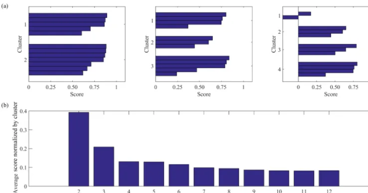
Figure 3.(a)Scores for each cluster analysis of observational data in the North Atlantic fork=2,k=3,k=4, where clusterkis the predetermined number of clusters and each bar represents the score per 2-D histogram.(b)Average scores for each cluster analysis with increasingk, fromk=2, . . .,12, normalized by the number of clustersk.
2015), where the average radius of each cluster (the distance from the centroid to the most distant member within a clus-ter) is computed for decreasingk. Bankert and Solbrig (2015) found that when the number of clusters falls below the opti-malk, the average radius grows rapidly. We employ a simi-lar methodology here. First, we use a scoring algorithm that computes the distance of each 2-D histogram from the cen-troid of its cluster. The higher the score is, the closer the 2-D histograms are to the centroid. The maximum score is 1, which indicates a perfect match. Negative or low values indi-cate poorly matched histograms that are the farthest from the centroid in the cluster. We run the scoring algorithm fork=2 throughk=12, since we have 12 2-D histograms, and there-fore there can be up to 12 clusters. Figure 3a shows the scores only fork=2,k=3, andk=4 as examples of the output of the scoring algorithm. We find that fork=2 and k=3 all 2-D histograms are well matched within a cluster (i.e., all scores are high), whereas fork=4 there is 1 month with a negative score. To further summarize the scoring results, we introduce a “sensitivity criterion” to the predetermined num-ber of clusters,k, in which we average all scores for eachk and normalize byk. The results are shown in Fig. 3b, where we note that the averaged normalized score fork=2 is 0.4, and it then quickly drops to 0.2 fork=3 and to 0.1 fork=4, and it plateaus after that. We choose as the optimal number of clusters thekwith the highest score and no significant change in the normalized averaged score thereafter. This choice im-plies that any reorganization of the 2-D histograms within more than three clusters will not produce any “tighter” clus-ters, i.e., clusters where the members are closer together. We must note here that the method is not entirely objective, as one always needs to visually inspect the clusters themselves and ensure that the choice ofkis indeed the best one.
3.4 Data normalization
As noted earlier,pCO2and SST have a broad range of
val-ues. Specifically, pCO2 values vary by about 2 orders of
magnitude between 50 and 450 uatm, and SST by 1 order of magnitude between−2 and 30◦C. It is customary in ap-plications of statistical techniques such as clustering to nor-malize the data (subtract the mean and divide by the standard deviation) in order to force both datasets to be in the same range of values. However, this is not always necessary (An-derberg, 1973, p. 13; Kaufman and Rousseauw, 2005, p. 11). In our case, we are not clustering each variable separately in order to determine regression coefficients (as in Lefèvre et al., 2005). Rather, we are clustering the 2-D histograms and comparing them, in order to obtain groups of similar patterns. In addition, clusters represented in normalized data are not as easily understood physically and as well represented on ge-ographical maps. Therefore we choose not to normalize the data for the purposes of this study.
4 Results
4.1 The North Atlantic Ocean carbon states
Figure 4 depicts the regimes for k=2, k=3, and k=4. When only two clusters are predefined, i.e., fork=2, the first cluster (Regime 2A, Fig. 4a) is dominated (30 % of the time) by pCO2-SST pairs in the ranges of 350–400 uatm
and 25–30◦C. The second cluster (Regime 2B) is dominated (20 %) bypCO2 swvalues within 300–350 uatm and SST
Figure 4.Cluster analysis output (regimes) for(a)k=2,(b)k=3, and(c)k=4 for the North Atlantic, from the Takahashi observational dataset. The color bar represents the relative frequencies of occurrence of each value-pair interval; i.e., the frequencies are divided by the total number of frequencies per regime.
frequencies. Regime 3A is a new state that was unresolved in k=2, but is not similar to 3B or 3C. Fork=4, Regimes 4B and 4C appear to be almost equivalent, and both derived from Regime 3B, which probably indicates that there is no new in-formation gained by requiring four clusters. Similar visual inspection of the results fork >4 confirms our more objec-tive analysis result thatk=3 is the optimal number of clus-ters in the pCO2-SST space in the North Atlantic basin. It
should be noted here that because we implementkclustering in the 2-D histograms and not the raw data, there is really no change in the results if we use a different number of bins in the histograms or if we use normalized data.
4.2 Temporal attribution for the North Atlantic carbon states
In order to characterize the ocean carbon states obtained in the previous section, we perform a temporal attribution anal-ysis by determining when each cluster occurs. This is possi-ble because for each cluster (regime), thek-means analysis routine computes the distance of every 2-D histogram in that cluster to the cluster’s centroid. Since each 2-D histogram is associated with a certain month in the climatology, we are able to associate each cluster with certain months. Fig-ure 5b shows that in the North Atlantic basin, regime 1 is represented by months January, February, March, and April and we call this the “winter regime”; regime 2 occurs dur-ing June, July, August, September and October and we will thus call it the “summer regime”; regime 3 occurs in May, November, and December and we will call this the
“transi-tion regime” because it reflects a mixed season in between the winter and summer regimes. Not surprisingly, these re-sulting regimes align themselves fairly well with the boreal winter and summer seasons in the North Atlantic. The cold season (winter regime) includes March and April but not November–December, which are included, rather, in the tran-sition regime. The warm season (summer regime) includes the months between June and October, again broader than the typical boreal summer. It is not surprising that we recover the seasonal cycle from the 12-month climatology, and probably because our domain is the entire North Atlantic, from the Equator to the subpolar regions, these seasons are broader including months from the spring and fall, since the length of each season is different at different latitudes.
4.3 Spatial attribution of the North Atlantic carbon states Next, we describe the geographical distribution of each regime (Fig. 5c). To do so, the frequencies of occurrence as-sociated with each pCO2-SST bin in Fig. 5a are averaged
over the months in each regime and mapped on the North At-lantic basin. We find that in the winter regime, the dominant value pairs (300–350 uatm and 10–20◦C) are found in the subtropical North Atlantic. In contrast, the dominant range of pCO2-SST pairs in the summer regime occurs in the tropics
(values 350–400 uatm and 25–30◦C). The transition regime shows a mix of the winter and summer regimes.
We conclude that the ocean carbon states determined by a 12-month climatology of surface oceanpCO2 and SST are
Figure 5.(a)Ocean carbon states (regimes) in observation-based data of the North Atlantic.(b)Monthly attribution of each ocean carbon regime in the Takahashi observational dataset. Temporal attribution is based on the distance of each monthly 2-D histogram to the centroid of each cluster. Each color represents a different regime: blue denotes the cold months’ regime (winter regime), red the warm months (summer regime) and green the May/November–December transition regime, since this is more a mix of the other two.(c)Regional attribution of each regime depicted in(a). The colors in(c)correspond to the ones in(a), i.e., to the frequencies of occurrence of each bin (value pair) in the clusters of(a).
pairs occur in the subtropical North Atlantic and the subpo-lar region. In the warm season, however, the most persistent value pairs occur in the tropical Atlantic. For more complex datasets, e.g., when interannual variability is included, we ex-pect to be able to detect regimes that correspond to processes controlled by the El Nino–Southern Oscillation (ENSO) or the North Atlantic Oscillation, for example.
4.4 The NASA-GISS climate model North Atlantic carbon states
Next we obtain the ocean carbon states from the GISS model simulations, following here the same methodology as for the observations. We are interested in understanding how similar the model regimes are to the observed ones we found earlier. As described in Sect. 2.3, we construct the ensemble mean climatologies forpCO2 swand SST for the period 1995–2005
from five simulations of Earth’s historical climate of the 20th century performed with the NASA-GISS climate model. We then obtain the 12-monthly 2-D histograms from the model climatology and, using the same binning groups as in the ob-servations, we obtain the model clusters. It should be noted here again that because we are actually clustering the 2-D histograms and not the raw data, our clusters are not sensi-tive to the number of bins or to normalization of the datasets prior to cluster analysis.
The sensitivity criterion (discussed in Sect. 3) for the model clusters is not as clear as in the case of the observa-tions (Fig. 6). Note that there is a plateau afterk=5 and thus it appears that 5 would be a more suitable choice fork. How-ever, as seen in Fig. 6a, some of the additional regimes in-clude only one monthly 2-D histogram. We therefore chose herek=3, recognizing that the model clusters have larger uncertainty. In a larger dataset that includes interannual vari-ability, more than a single 2-D histogram would potentially be assigned to a regime, reducing that uncertainty.
Figure 7a shows the ocean carbon states fork=3, while Fig. 7b characterizes their temporal occurrence: the model winter regime corresponds to the months December, January, February, March, April, and May; the summer regime corre-sponds to the months July, August, September, October, and November; the transition regime corresponds only to June. There is therefore good agreement with the regimes from observations (Fig. 5b). The model winter regime is some-what broader than that observed by 2 months (December and May), while the model summer regime lags by 1 month (starts in July, while in the observations it starts in June).
Figure 6.(a)Scores for each cluster analysis of the GISS model data in the North Atlantic fork=2,k=3,k=4,k=5, where clusterkis the predetermined number of clusters and each bar represents the score per 2-D histogram.(b)Average scores for each cluster analysis with increasingk, normalized by the number of clustersk.
Figure 7.(a)Ocean carbon states (regimes) in the North Atlantic from the GISS model output.(b)Monthly attribution of each ocean carbon regime. Temporal attribution is based on the distance of each monthly 2-D histogram to the centroid of each cluster. Blue denotes the cold month regime (winter regime), red the warm months (summer regime) and green the transition regime (only June), since this is more a mix of the other two.(c)Regional attribution of each regime depicted in(a). The frequencies of occurrence of each bin (value pair) in the clusters of(a)are mapped onto the North Atlantic grid.
in the range of 300–350 uatm and 20–25◦C, at 30 and 25% relative frequency. However, other weaker pairs are not well represented in the model, e.g., the range 50–200 uatm and−2 to 10◦C. During the winter regimes, the highest frequency of occurrence (25 %) is for the pair of values 300–350 uatm and 10–20◦C, whereas in the model the same pair of values is found 30 % of the time. Similarly, the summer and tran-sition regime highest frequency pairs are well simulated. In
contrast, the value pairs 200–350 uatm for very cold temper-atures are not well represented in the model.
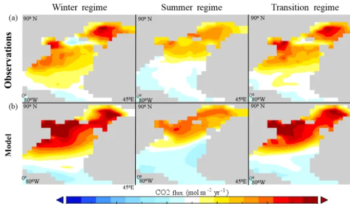
Figure 8.Composites of the CO2flux field over the observed regimes for(a)the observations and(b)the model. The composite fields are
computed as averages of the field over the months included in each regime. Both the observations and the model data are composited over the same months as determined by the temporal attribution of the observations dataset, shown in Fig. 5b. Blue shades indicate outgassing, and red shades indicate uptake.
Fig. S2). In contrast, the dominant range ofpCO2-SST pairs
in the summer regime occurs in the tropics (values 350– 400 uatm and 25–30◦C; Fig. 7c) and is of higher frequency in the observations than the model. In other words, the model underestimates the extent of the tropical summer regime but reproduces well the other parts of the summer regime. The transition regime shows a mix of the winter and summer regimes for both observations and model. The model results in this regime indicate higher frequency in the subpolar re-gion than in the observations.
4.5 Model North Atlantic air–sea flux of CO2error
analysis and bias attribution
The ocean carbon states can provide a framework for model assessment against the observations. In this section we seek to identify biases in the simulated flux of CO2and attribute
them to leading biases in physical and biogeochemical pro-cesses.
In the previous section we used the same methodology as in the observations to obtain independently the model regimes and assess how different they are. However, when we want to identify the causes of the model biases, we have to use the observed regimes as the basis of the comparison and assign the model data to the observed regimes, by averaging the model data over those months that the observed regimes occur (Fig. 5b). This approach was highlighted in Williams and Webb (2009) for general circulation model evaluations of the cloud regimes.
Figure 8 depicts the air–sea flux of CO2composited over
the observed temporal regimes in both observations (Fig. 8a) and model output (Fig. 8b). In the winter regime, model
out-gassing (in shades of blue) is confined only to the tropics, whereas in the observations there is also a tongue of out-gassing at about 60◦N. Similarly, in the transition regime, the model has a more extended uptake region in the subpolar North Atlantic than in the observations. While the summer regime is better represented in the model than the other two regimes, all three regimes show that model uptake is stronger than in observations at mid and high latitudes and that out-gassing is also stronger in the model at mid to low latitudes.
To trace the source of model biases in the air–sea flux of CO2we need a better understanding of the physical or
bio-geochemical processes that control the air–sea flux of CO2
in the model. Using the clustering analysis results from the previous section, we can investigate the underlying processes that might be responsible for the bias.
The process attribution is performed using a Taylor expan-sion of the model bias as shown in Eq. (5). The model flux bias,1F, depends on the biases of pCO2 sw, SST, salinity
(SSS) and wind speed (wspd) such that
1F ∼ ∂F
∂pCO2 sw
1pCO2 sw+ ∂F ∂SST1SST
+ ∂F
∂SSS1SSS+ ∂F
∂wspd1wspd, (5)
where 1q is the bias of the variable q, defined as the root mean squared error (RMSE) between the observa-tions and the model, and q is any of the variables {pCO2 sw,SST,SSS,wspd}. ∂F∂q is a weight term that
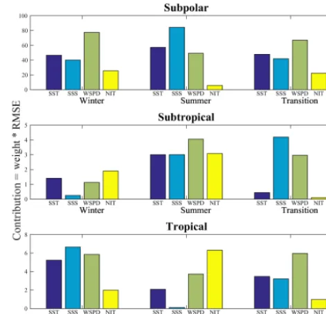
merid-Figure 9.Contributions of each of the variablespCO2, SST, SSS,
and WSPD to the overall air–sea flux1F bias. The contributions are computed as the products of the weights and the RMSEs of each variableqas described in Eq. (5). See the text for a detailed expla-nation.
ionally, and because the carbon states’ regional distribution (Fig. 5c) is quite complex, we identify areas where the linear fits will be more appropriate approximations of the {F, q} relationships. The subpolar region where the value pairs are −2 to 10◦C and 50 to 350 uatm, a subtropical region (10 to 20◦C, 300 to 350 uatm), and a tropical region (20 to 30◦C, 300 to 400 uatm) are demarcated in Fig. S2. Results of the regional scatter plots and the linear fit for each regime are shown in Fig. S3 and are synthesized in Fig. 9. Each contribu-tion term (each term on the right-hand side of Eq. 5) is calcu-lated from the multiplication of the weights and the RMSEs. Figure 9 then shows that over most of the North Atlantic, the flux biases are attributed mainly to errors in thepCO2 sw,
although in subpolar regions other terms such as salinity bi-ases and wind speed bibi-ases become important. It therefore makes sense to further investigate biases inpCO2 swand the
processes these are attributed to, as presented in Eq. (2). Similarly to Eq. (5),
1pCO2 sw∼
∂pCO2 sw
∂SST 1SST+
∂pCO2 sw ∂SSS 1SSS
+∂pCO2 sw
∂WSPD 1WSPD+
∂pCO2 sw
∂NITRATE1NIT. (6)
We perform the Taylor expansion of the bias for each of the regimes that we computed, calculating the weights and RM-SEs in the same way as described for CO2flux biases. The
estimates of the linear fit slopes of the scatter plots are shown in Fig. S4 and the composites of the contributions in Fig. 10.
Figure 10.Contributions to thepCO2 sw bias in the model from
SST, SSS, wind speed (WSPD) and nitrate (NIT) in the winter, summer, and transitional regimes. Contributions are computed as in Fig. 9 (see details in the text). The entire North Atlantic is dif-ferentiated into subpolar, subtropical, and tropical regions to better account for regional differences in the model biases and obtain a better linear fit for the computation of the weights in Eq. (6).
Overall Fig. 10 shows that the biases in the subpolar region are larger than anywhere else in the North Atlantic basin, as the contributions to the bias inpCO2 sware an order of
mag-nitude larger there. Specifically, in the subpolar region, wind speed biases emerge as responsible for the winter and tran-sition regime biases inpCO2 sw, while salinity biases
dom-inate the summer bias inpCO2 sw. In the winter and
tran-sitional months, the quasi-cyclonic subpolar gyre, driven by energetic winds and wind outbreaks, leads to Ekman diver-gence in the surface layer that controls thepCO2 sw biases
near the coast. At the same time, winter-time convective mix-ing is responsible for biases in the strength of the Merid-ional Overturning Circulation that are known to influence open oceanpCO2 sw(Romanou et al,. 2017). In the summer
regime, GISS model sea-ice concentration is higher than ob-served; hence, melting will lead to significant surface salin-ity biases. Inaccurate model representation of the magnitude and fluctuations of the cyclonic wind stress curl as well as the sea-ice retreat and associated salinity changes are proba-bly responsible for deficient physical characterization of the model ocean circulation, which would result in misrepresen-tations of thepCO2 swand thus the CO2flux in the model.
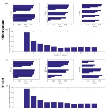
Figure 11.(a)Scores for each cluster analysis fork=2,k=3,k=4 for the observational data in the Southern Ocean where clusterkis the predetermined number of clusters and each bar represents the score per 2-D histogram.(b)Average scores of each clustering analysis for increasingk, fromk=1 tok=12.(c)Scores for each cluster analysis fork=2,k=3,k=4 for the model data in the Southern Ocean.
(d)Average scores of each clustering analysis for increasingk.
the surface by anticyclonic circulation and a strong western boundary current, the Gulf Stream. Gyre subduction supports downwelling which brings nutrients andpCO2to depth.
Ni-trate utilization by ocean biology during the winter regime is probably inaccurate in the model, while wind speed biases are known to be larger in the summer than the winter regime in the model.
In the tropics, biases in wind speed, nitrate and salinity are again found to be important. Here, nitrate biases, which are relatively higher in oligotrophic regions (Arteaga et al,. 2015), are probably due to misrepresentation of nitrogen fix-ation in the GISS climate model. Wind speed and salinity biases are associated with well-known biases in the intensity and position of the Inter Tropical Convergence Zone (ITCZ) that controls cloudiness, temperature gradient, and rainfall. The ITCZ moves north in the summer and south in the win-ter; therefore, a wind speed bias in the transition regime in the model could be explained by an inaccurate model reproduc-tion of how the ITCZ affects the wind during its transireproduc-tional
movement. The ITCZ increases precipitation, thus decreas-ing salinity; therefore, how salinity changes by season as a result of the shifting ITCZ could explain the winter regime bias.
4.6 The Southern Ocean carbon states
The application of cluster analysis in the Southern Ocean is presented here similarly to in the North Atlantic, with the purpose of examining whether the technique will also be able to identify some known aspects of the Southern Ocean carbon cycle. For brevity, though, the observation-based and model regimes will be presented alongside one another and will be followed by the model-error attribution analysis.
As done for the North Atlantic basin, we look at proba-bility density distributions of observations in the Southern Ocean which show that both SST and pCO2 sw exhibit a
12-based on Fig. 11c and 11d, which show that this is also the optimal number of clusters. There is added ambiguity in the choice ofkhere, in addition to that due to the small dataset, which arises from the fact that the Southern Ocean is a very broad basin zonally and different processes become impor-tant in different regions more so than in the narrow North Atlantic basin, which make the choice ofknot as clear as it was in the North Atlantic.
The observed and model ocean carbon states are shown in Fig. 12. In the summer regime, which includes January, February and March (see Fig. 13 and the explanation below), the highest frequency pair values (i.e., the most persistent pairs) are found around 20 % of the time in the observations and 25 % of the time in the model for the ranges of 250– 350 uatm and 0–5◦C. Another range of pair values which also shows a high frequency of occurrence (25 %) is found for warmer temperatures (10–20◦C) and the same range of pCO2, but the GISS model misplaces it towards higher
val-ues ofpCO2(350–400 uatm). The winter regime comparison
shows that the model captures the lowpCO2, low
tempera-ture state (20–150 uatm,−3 to 0◦C) well (30 % of the time in observations and in the model). The mid-rangepCO2, high
temperature state (250–350 uatm, 10–20◦C) is not as well represented in the model. The observations there show the highest frequencies of occurrence for higher pCO2 (350–
400 uatm), in contrast to the model for lower pCO2 (250–
350 uatm). Comparison between the transition regimes re-veals much less correspondence between observations and the GISS model, considering the high frequency states in ob-servations are quite different than in the model (e.g., obser-vations of high frequency states: 20–150 uatm, −3 to 0◦C; 250–350 uatm, 10–20◦C; 350–400 uatm, 0–5◦C; model high frequency state: 250–350 uatm, 0–10◦C).
4.6.1 Temporal attribution for the Southern Ocean carbon states
Temporal attribution, which is estimated using the method described in Sect. 4.1, is shown for both the model and the observations in Fig. 13. Note that all subsequent analysis
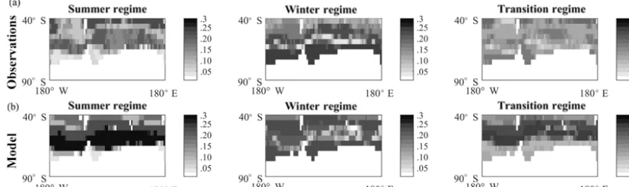
rence of each bin in the cluster are mapped onto the South-ern Ocean regions (Fig. 14), where geographic nomenclature similar to that in Orsi et al. (1995) is used. In the coastal Antarctic divergence zone, SST varies within −3 to 3◦C andpCO220–250 uatm, in the Antarctic convergence zone
SST ranges within 3–10◦C andpCO2250–400 uatm, and in
the subtropical convergence zone SST lies within 10–20◦C andpCO2250–400 uatm. Despite the strong temporal
attri-bution agreement between the model and the observations, the regional attributions show much less correspondence. For example, in the summer regime, the observations show the highest frequency of occurrence between 250–350 uatm and 10–20◦C along the subtropical convergence zone (roughly along 40◦S), while the highest frequency of occurrence for the model is for the pair 250–350 uatm and 0–5◦C, occur-ring in the coastal region (poleward of the divergence zone along 60◦S). In the winter regime, both observations and the GISS model show the highest frequency of occurrence for the value pairs nearest to the coast where thepCO2 is
low and the temperatures coldest (20–150 uatm and −3 to 10◦C). Further offshore, the model highest frequency val-ues occur for lowerpCO2 (250–350 uatm) than in the
ob-servations (350–400 uatm). Lastly, in the transition regime, the model shows a much higher persistency of values in the range (250–350 uatm and 0–10◦C) than in the observations.
It is therefore evident that the GISS model does not re-produce well the observed ocean carbon states in the South-ern Ocean. There is a tendency to persistently underestimate pCO2-SST values closer to the coast and overestimate it near
the subtropical convergence zone, during the warm season, whereas, during the cold season, the model captures well the divergence zone regime but the errors further offshore switch: the model now overestimatespCO2-SST value-pair
Figure 12.Comparison between the regimes in(a)the observations and(b)the model output.
Figure 13. Monthly attribution of each ocean carbon regime in observations and the GISS climate model. Temporal attribution is based on the distance of each monthly 2-D histogram to the cen-troid of each cluster. Referring to austral seasons, blue denotes the cold month regime (winter regime), red the warm months (summer regime) and green the transition regime, since this is more a mix of the other two.
4.6.3 Model Southern Ocean air–sea flux of CO2error analysis and bias attribution
Comparing the CO2flux composites on the observed regimes
(Fig. 15) shows significant discrepancies between observa-tions (Fig. 15a) and model (Fig. 15b). To better understand where these discrepancies come from, we perform an error attribution analysis, as in Sect. 4.1 above. In the summer regime (January through March), outgassing in the model is restricted to the subtropical convergence zone, whereas in the observations it is more localized and closer to Antarctica. At the same time, model uptake is stronger, confined to the coast and over a broader area than in the observations. This is con-sistent with the result from the previous section, where the model underestimatespCO2 and SST in the Antarctic
con-vergence zone. In the winter regime (June through October), the entire model basin is a sink for CO2, whereas in the
ob-servations there is a zonally confined outgassing belt south of 50◦S and an uptake belt north of it. Again, this result is con-sistent with the earlier finding that the model winter regime is closer to the observed near the Antarctic coast. The
transi-tion regime shares a mix of the same discrepancies as in the summer and winter regimes.
Bias attribution is computed for the three zonally defined regions indicated in Fig. S6. Based on the bias computations in Eq. (5) forpCO2 sw, SST, salinity, and wind speed with
respect to CO2flux,pCO2 swis again shown to be the
driv-ing variable in most of the flux biases in the Southern Ocean (Fig. S7; Fig. S8 for scatter plots). We therefore seek to un-derstand the processes that control the pCO2 biases in the
model, using the Taylor expansion in Eq. (6) (Fig. 16; Fig. S9 for scatter plots).
rel-identified by the observations’ temporal attribution.
Figure 15.Composites of the CO2flux field over the regimes in the Southern Ocean for(a)the observations and(b)the GISS model. Both the observations and the model data are composited over the same months as determined by the temporal attribution of the observed regimes. Blue shades indicate outgassing, and red shades indicate uptake.
atively very important in the region south of the subtropical convergence zone, which suggests that a study of water mass formation in that region in the model and the observations would better explain the biases.
5 Data availability
Data and analysis scripts can be accessed at https://data.giss. nasa.gov/oceans/carbonstates.
6 Conclusions
This proof-of-concept study presents the k-means cluster analysis and the determination of the regimes called “ocean
carbon states” in observation-based data of the ocean car-bon cycle. A method is described here to determine the op-timal number of clusters for the cluster analysis. The study also explores how to characterize the ocean carbon states temporally and spatially in order to determine the physical– biogeochemical processes related to each carbon state. Com-posites of the CO2flux and a quantitative exploration of the
effect of each field onpCO2 swbias are also demonstrated.
In this study,pCO2and SST were chosen as the two
vari-ables that co-determine the carbon states, based on the fact that they both play critical roles in the biogeochemistry and the physics of the ocean system and control the flux of CO2.
interest-Figure 16.Contributions to thepCO2 sw bias in the model from
SST, SSS, wind speed (WSPD) and nitrate (NIT) in the winter, sum-mer, and transitional regimes. The Southern Ocean is differentiated into the coastal Antarctic divergence zone (roughly polewards of 60◦S), Antarctic convergence zone (roughly 60–50◦S), and sub-tropical convergence zone (roughly 50–40◦S) to better account for regional differences in the model biases and obtain better linear fit for the computation of the weights in Eq. (6) (see Fig. S9).
ing to see whether and how the regimes depend on the choice of variables.
We have also tested the importance of the choice ofk. A main caveat of k-means cluster analysis is that k must be predetermined through reasoning that is subject to personal bias. However, we show that by assessing the clusters from multiple angles (i.e., the score plots, the sensitivity criterion visual inspection, analysing cluster outputs with increasingk, temporal attribution), it is possible to determine an optimalk that is semi-objective. Even so, in this proof of concept study, we acknowledge the uncertainty in our choice ofkas a result of the small dataset of 12-monthly 2-D histograms, which occasionally results in there being only a small number of histograms per cluster.
The ocean carbon states we obtain from this climatolog-ical year dataset are interesting. We found that the subtrop-ical North Atlantic is the dominant feature in the cold sea-son regime (the months January through April). In the same regime, the subpolar North Atlantic also features promi-nently, which is associated with the high variability in this area due to sea ice retreat, the spring bloom and the winter– spring convection. In contrast, the tropical Atlantic domi-nates the warm months June through October, while the sub-tropical and subpolar regions play a smaller role. The tran-sition regime, which is comprised of months that do not en-tirely fall into the winter or summer regimes, shows again
the lower tropics and the subtropical gyre to be more active. We would expect that a longer dataset that includes natural variability as well as the effects of longer-term climate and anthropogenic trends would result in more carbon states and hence that it would be an interesting extension of the present study.
The NASA-GISS model carbon states in the North At-lantic are similar, both in temporal as well as spatial char-acterization, to the observed ones, with better model skill in the summer than in the winter. Specifically, the model over-estimates the importance of the subtropical gyre and under-estimates the subpolar gyre during the cold months. During summer, the model underestimates the tropics, but not signif-icantly. The transition months are found to behave differently in the model, although that might be a result of the small size of our input datasets.
In the Southern Ocean, during the warmer months (January–March), the observational states are more persis-tent along 40◦S, the subtropical convergence zone, while the colder season has prominent states (higher persistency) mostly along the Antarctic coast. The transition regime shows a similar degree of variability across the entire South-ern Ocean.
While the GISS model agrees in the temporal characteri-zation of the ocean carbon states, it diverges from the obser-vational spatial attribution, particularly in the summer and the transition regimes. It is of note here, however, that the Takahashi climatology is far more uncertain in the Southern Ocean (Takahashi et al., 2009) than it is in the North Atlantic, and therefore the model’s lack of skill might not be as alarm-ing. New observations in the area (e.g., from SOCCOM) will greatly benefit studies such as this.
Error analysis of the model response helps explain the GISS model biases. Applying k-means clustering analysis in the two main regions of the world that are known to be critical for the global ocean carbon cycle, namely the North Atlantic region and the Southern Ocean, defines the priorities for model improvement: in the North Atlantic biases in sur-face salinity, wind speed and sursur-face temperature, whereas in the Southern Ocean priorities are nitrate and surface salinity. Clearly the GISS climate model would benefit from more re-alistic representation of the nitrogen cycle in the ocean as a whole.
The goal of this study is to enable us to apply thisk-means clustering to “big” data, in order to find the interannual and regional patterns in larger, higher frequency climate datasets. This extended application will allow researchers to gain a much more comprehensive insight and intuition for physical systems by mechanistically and impartially grouping multi-ple variables that form the prominent features of these net-works. Other variable pairs besidespCO2and SST will also
be explored, such as CO2 flux and chlorophyll, in order to
Acknowledgements. Resources supporting this work were pro-vided by the NASA High-End Computing (HEC) program through the NASA Center for Climate Simulation (NCCS) at Goddard Space Flight Center.
Funding was provided by NASA-ROSES Modeling, Analy-sis and Prediction 2013 NNX14AB99A-MAP for GISS Model-E development and NNX15AJ05A NASA Cooperative Agreement 2015–2018.
Data used to generate figures, graphs, plots, as well as analysis were archived at the NCCS dirac repository, numerical codes are maintained and archived at GISS and all data and codes are available upon request from Anastasia Romanou. Clustering analysis was performed using the MATLAB ver 2015 computing environment. The authors wish to thank Robert Schmunk for his help in setting up the Zenodo page and the GISS portal.
Edited by: David Carlson
Reviewed by: Lionel Arteaga and two anonymous referees
References
Anderberg, M. R.: Cluster analysis for applications, Academic Press, New York, 1973.
Arteaga, L., Pahlow, M., and Oschlies, A.: Global monthly sea surface nitrate fields estimated from remotely sensed sea surface temperature, chlorophyll, and modeled mixed layer depth, Geophys. Res. Lett, 42, 1130–1138, https://doi.org/10.1002/2014GL062937, 2015.
Bankert, R. L. and Solbrig, J. E.: Cluster Analysis of A-Train Data: Approximating the Vertical Cloud Structure of Oceanic Cloud Regimes, J. Appl. Meteorol. Clim., 54, 996–1008, https://doi.org/10.1175/JAMC-D-14-0227.1, 2015.
Bodas-Salcedo, A., Williams, K. D., Ringer, M. A., Beau, I., Cole, J. N., Dufresne, J., Koshiro, T., Stevens, B., Wang, Z., and Yokohata, T.: Origins of the Solar Radiation Biases over the Southern Ocean in CFMIP2 Models, J. Climate, 27, 41–56, https://doi.org/10.1175/JCLI-D-13-00169.1, 2014
Boyer, T. P., Antonov, J. I., Baranova, O. K., Coleman, C., Gar-cia, H. E., Grodsky, A., Johnson, D. R., Locarnini, R. A., Mishonov, A. V., O’Brien, T. D., Paver, C. R., Reagan, J. R., Seidov, D., Smolyar, I. V., and Zweng, M. M.: World
Clustering (MSTC) as a data mining tool for environmen-tal applications, edited by: Sànchez-Marrè, M., Bìejar, J., Co-mas, J., Rizzoli, A. E., and Guariso, G., Proceedings of the iEMSs Fourth Biennial Meeting: International Congress on En-vironmental Modelling and Software Society (iEMSs 2008), Barcelona, Catalonia, Spain, July 2008.
Hoffman, F. M., Larson, J. W., Mills, R. T., Brooks, B. J., Ganguly, A. R., Hargrove, W. W., Huang, J., Kumar, J., and Vatsavai, R. R.: Data Mining in Earth System Sci-ence (DMESS 2011), Procedia Comput. Sci., 4, 1450–1455, https://doi.org/10.1016/j.procs.2011.04.157, 2011.
Hugue, F., Lapointe, M., Eaton, B. C., and Lepoutre, A.: Satellite-based remote sensing of running water habitats at large riverscape scales: Tools to analyze habitat heterogeneity for river ecosystem management, Geomorphology, 253, 353–369, https://doi.org/10.1016/j.geomorph.2015.10.025, 2016. Jain, A. K.: Data clustering: 50 years beyond
K-means, Pattern Recogn. Lett., 31, 651–666, https://doi.org/10.1016/j.patrec.2009.09.011, 2010.
Jakob, C. and Tselioudis, G.: Objective identification of cloud regimes in the Tropical Western Pacific, Geophys. Res. Lett., 30, 2082, https://doi.org/10.1029/2003GL018367, 2003.
Johnson, K. S., Plant, J. N., Coletti, L. J., Jannasch, H. W., Sakamoto, C. M., Riser, S. C., Swift, D. D., Williams, N. L., Boss, E., Haentjens, N., Talley, L. D., and Sarmiento, J. L.: Biogeochemical sensor performance in the SOCCOM pro-filing float array, J. Geophys. Res.-Oceans, 122, 6416–6436, https://doi.org/10.1002/2017JC012838, 2017
Kaufman, L. and Rousseauw, P.: Finding Groups in Data: An Intro-duction to Cluster Analysis, John Wiley & Sons, Inc., Hoboken, New Jersey, 2005.
Landschützer, P., Gruber, N., Bakker, D. C. E., Schuster, U., Nakaoka, S., Payne, M. R., Sasse, T. P., and Zeng, J.: A neu-ral network-based estimate of the seasonal to inter-annual vari-ability of the Atlantic Ocean carbon sink, Biogeosciences, 10, 7793–7815, https://doi.org/10.5194/bg-10-7793-2013, 2013. Landschützer, P., Gruber, N., Bakker, D. C. E., and
Schuster, U.: Recent variability of the global ocean carbon sink, Global Biogeochem. Cy., 28, 927–949, https://doi.org/10.1002/2014GB004853, 2014.
for mapping in situ pCO2 data, Tellus B, 57, 375–384,
https://doi.org/10.1111/j.1600-0889.2005.00164.x, 2005. Nakaoka, S., Telszewski, M., Nojiri, Y., Yasunaka, S., Miyazaki, C.,
Mukai, H., and Usui, N.: Estimating temporal and spatial varia-tion of ocean surfacepCO2in the North Pacific using a
self-organizing map neural network technique, Biogeosciences, 10, 6093–6106, https://doi.org/10.5194/bg-10-6093-2013, 2013. Oreopoulos, L., Nayeong, C., Lee, D., and Kato, S.: Radiative
ef-fects of global MODIS cloud regimes, J. Geophys. Res., 121, 2299–2317, https://doi.org/10.1002/2015JD024502, 2016. Orsi, A., Whitworth, T., and Nowlin, W. D.: On the meridional
ex-tent and fronts of the Antarctic Circumpolar Current, Deep-Sea Res. Pt. I, 42, 641–673, 1995.
Peron, T. K. D., Comin, C. H., Amancio, D. R., da F. Costa, L., Rodrigues, F. A., and Kurths, J.: Correlations between climate network and relief data, Nonlin. Processes Geophys., 21, 1127– 1132, https://doi.org/10.5194/npg-21-1127-2014, 2014. Phillips, J. D., Schwanghart, W., and Heckmann, T.: Graph
theory in the geosciences, Earth-Sci. Rev., 143, 147–160, https://doi.org/10.1016/j.earscirev.2015.02.002, 2015.
Radebach, A., Donner, R. V., Runge, J., Donges, J. F., and Kurths, J.: Disentangling different types of El Niño episodes by evolving climate network analysis, Phys. Rev. E, 88, 052807, https://doi.org/10.1103/PhysRevE.88.052807, 2013.
Romanou, A., Gregg, W. W., Romanski, J., Kelley, M., Bleck, R., Healy, R., Nazarenko, L., Russell, G.. Schmidt, G. A., Sun, S., and Tausnev, N.: Natural air–sea flux of CO2 in
simu-lations of the NASA-GISS climate model: Sensitivity to the physical ocean model formulation, Ocean Model., 66, 26–44, https://doi.org/10.1016/j.ocemod.2013.01.008, 2013.
Romanou, A., Marshall, J., Kelley, M., and Scott, J.: Role of the ocean’s AMOC in setting the uptake efficiency of transient tracers, Geophys. Res. Lett., 44, 5590–5598, https://doi.org/10.1002/2017gl072972, 2017.
Rossow, W. B., Zhang, Y.-C., and Wang, J.: A statistical model of cloud vertical structure based on reconciling cloud layer amounts inferred from satellites and radiosonde humidity profiles, J. Cli-mate, 18, 3587–3605, https://doi.org/10.1175/JCLI3479.1, 2005. Sarmiento, J. L. and Gruber, N.: Ocean Biogeochemical Dynamics,
Princeton University Press, New Jersey, USA, 2006.
Sasse, T. P., McNeil, B. I., and Abramowitz, G.: A new constraint on global air–sea CO2fluxes using bottle carbon data, Geophys.
Res. Lett., 40, 1594–1599, https://doi.org/10.1002/grl.50342, 2013.
Takahashi, T., Sutherland, S. C., Wanninkhof, R., Sweeney, C., Feely, R. A., Chipman, D. W., Hales, B., Friederich, G., Chavez, F., Watson, A., Bakker, D. C. E., Schuster, U., Metzl, N., Yoshikawa-Inoue, H., Ishii, M., Midorikawa, T., Nojiri, Y., Sabine, C., Olafsson, J., Arnarson, Th. S., Tilbrook, B., Jo-hannessen, T., Olsen, A., Bellerby, R., Körtzinger, A., Stein-hoff, T., Hoppema, M., de Baar, H. J. W., Wong, C. S., Delille B., and Bates, N. R.: Climatological mean and decadal changes in surface ocean pCO2, and net sea-air CO2 flux over the global oceans, Deep-Sea Res. Pt. II, 56, 554–577, https://doi.org/10.1016/j.dsr2.2008.12.009, 2009.
Telszewski, M., Chazottes, A., Schuster, U., Watson, A. J., Moulin, C., Bakker, D. C. E., González-Dávila, M., Johannessen, T., Körtzinger, A., Lüger, H., Olsen, A., Omar, A., Padin, X. A., Ríos, A. F., Steinhoff, T., Santana-Casiano, M., Wallace, D. W. R., and Wanninkhof, R.: Estimating the monthlypCO2
distribu-tion in the North Atlantic using a self-organizing neural network, Biogeosciences, 6, 1405–1421, https://doi.org/10.5194/bg-6-1405-2009, 2009.
Trans Mills, R., Hoffman, F. M., Kumar, J., and Hargrove, W. W.: Cluster Analysis-Based Approaches for Geospatiotem-poral Data Mining of Massive Data Sets for Identification of Forest Threats, Procedia Comput. Sci., 4, 1612–1621, https://doi.org/10.1016/j.procs.2011.04.174, 2011.
Trochta, J. T., Mouw, C. B., and Moore, T. S.: Remote sensing of physical cycles in Lake Superior using a spatio-temporal analysis of optical water typologies, Remote Sens. Environ., 171, 149– 161, https://doi.org/10.1016/j.rse.2015.10.008, 2015.
Tselioudis, G., Rossow, W., Zhang, Y., and Konsta, D.: Global Weather States and Their Properties from Passive and Ac-tive Satellite Cloud Retrievals, J. Climate, 26, 7734–7746, https://doi.org/10.1175/JCLI-D-13-00024.1, 2013.
Wanninkhof, R.: Relationship between wind speed and gas ex-change over the ocean, J. Geophys. Res., 97, 7373–7382, https://doi.org/10.1029/92JC00188, 1992.
Wanninkhof, R., Park, G.-H., Takahashi, T., Sweeney, C., Feely, R., Nojiri, Y., Gruber, N., Doney, S. C., McKinley, G. A., Lenton, A., Le Quéré, C., Heinze, C., Schwinger, J., Graven, H., and Khatiwala, S.: Global ocean carbon uptake: magni-tude, variability and trends, Biogeosciences, 10, 1983–2000, https://doi.org/10.5194/bg-10-1983-2013, 2013.
Williams, K. and Webb, M.: A quantitative performance assessment of cloud regimes in climate models, Clim. Dynam., 33, 141–157, https://doi.org/10.1007/s00382-008-0443-1, 2009.
Wood, R., Wyant, M., Bretherton, C. S., Rémillard, J., Kollias, P., Fletcher, J., Stemmler, J., de Szoeke, S., Yuter, S., Miller, M., Mechem, D., Tselioudis, G., Chiu, J. C., Mann, J. A., O’Connor, E. J., Hogan, R. J., Dong, X., Miller, M., Ghate, V., Jefferson, A., Min, Q., Minnis, P., Palikonda, R., Albrecht, B., Luke, E., Hannay, C., and Lin, Y.: Clouds, Aerosols, and Precipitation in the Marine Boundary Layer: An Arm Mo-bile Facility Deployment, B. Am. Meteorol. Soc., 96, 419–440, https://doi.org/10.1175/BAMS-D-13-00180.1, 2015.