Analysis of Impedance Spectroscopy Data—Finding the Best System Function

Analysis of Impedance Spectroscopy Data—Finding

the Best System Function

SIOMA BALTIANSKI & YOED TSUR∗

Chemical Engineering Department, Technion—Israel Institute of Technology, Haifa 32000, Israel

Submitted February 5, 2003; Revised March 31, 2003; Accepted April 1, 2003

Abstract. Impedance spectroscopy gains much attention as a non-destructive analysis technique in many areas of materials science and device manufacturing. While it is relatively easy to collect data, the correct analysis or the data interpretation is not a straightforward task. In this paper, a novel analysis technique that provides a simple mean to identify the best system function is shown.

A new taxonomy of all the possible circuit models that are based on RC lumped elements is given. The taxonomy divides the various circuit models into groups of increasing complexity. Its order and family, where for RC elements there are four different families, identify each group. A “black box”, rather than a pre-assumed circuit model, represents the sample under test (SUT). The simplest group (order and family) that describes the SUT accurately within the experimental limitations can be found in a single experiment. In some cases, the best circuit model within the group can also be found by investigating the behavior of the SUT under various changes (i.e., temperature, radiation, other environmental conditions, sample construction, etc.).

The technique is demonstrated on various circuits with lumped capacitors and resistors. This is done both on actual systems and on synthetic data with artificial noise. A comparison of this method with a standard Cole-Cole identification demonstrates the power of the new approach.

Keywords: impedance spectroscopy, electrical properties, system identification, inverse problem

Introduction

The common practice of using impedance spectroscopy is to assume a circuit model first, and then to analyze the obtained experimental data according to the pre-assumption [1]. This pre-pre-assumption takes the form of a function, say Z(s) (where s≡iω), and the values

of its parameters are found by fitting—typically using complex nonlinear least squares [2, 3]. Further, in some cases the validity of the experimental results is checked using the Kramers-Kronig transforms [4, 5].

Can we identify the best circuit model, as part of the data analysis (“black box” attitude)? In answering this question, one has to address two problems. The first one is how to identify the best function for a given set of data (including errors). The second one is how to

∗_{To whom all correspondence should be addressed. E-mail:}

[email protected]

find the best equivalent circuit to describe the SUT for a given system function.

data to a Cole-Cole plot, the new approach identifies it correctly as 4th order 1st family. This final example demonstrates the power of the new approach.

Methods

Taxonomy of the System Functions in the RC Case

All the system functions describing circuit models that are based on lumped resistors and capacitors have the general form:

Z(s)=

iais i

ibisi

; s≡√−1·ω (1)

Moreover, there are only four different basic forms of this formula for the case of RC circuits, which we call families. Those families are:

                            

1. Z(s)= 1+ n−1

i=1 ais i

n i=1bisi

2. Z(s)= 1+ n₋1

i=1 ais i

b0+ni=1bisi

3. Z(s)= 1+ n

i₌1aisi

n i₌1bisi

4. Z(s)= 1+ n

i=1ais i

b0+ni=1bisi

(2)

The order of the system function is the rank of the de-nominator polynomial, and is the number of capacitors in the corresponding RC model circuits. Some special low order cases are (order, family): (0, 4) a resistor—

Z(s)=1/b0; (1, 1) a capacitor—Z(s)=1/b1s; (1, 2) parallel R and C—Z(s) = _b 1

0+b1s; (1, 3) R and C in

series—Z(s) = 1+a1s

b1s ; and (1, 4) a resistor in series

with parallel R and C—Z(s)= 1+a1s

b0+b1s. The last system

function (1, 4), is a system function of two different circuit models that produce the same impedance at all frequencies. This is the first group with more than one member. The number of circuit models per group grows rapidly with the number of independent parameters in the system function. The number of independent pa-rameters in the system function equals the number of elements (R and C) in the model circuit, and is 2n−1 for the first family, 2n for the second and third family and 2n+1 for the fourth family. Thus, the fourth family of ordern−1 is as complex as the first family in order

n while the second family is as complex as the third family in the same order.

How to Identify the Best Order and Family

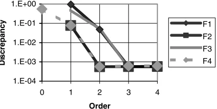
The “best” system function would be the one that can reproduce the experimental data within the error level of the measurement system with the least number of components. For each system function, after fitting and finding the relevant parameters [6], one can find the discrepancy by calculating the variance. The weight-ing function should not be in general the best one for fitting the system parameters. It should rather be a “less forgiving” weighting function, to get a clear kinks in the plot described below. For most cases that we have investigated, unit weighting is the most convenient one for this purpose. The logarithm of the discrepancy is then plotted for each family against the order. This re-sults typically in a straight line with a sharp kink in a certain order and variance that corresponds to the noise level of the experiment. These kinks can show up in different orders for different families. The best order is chosen as the lowest order with a kink, simply because increasing the order (and complexity) does not reduce the discrepancy. If more than one family have their kinks at the same order, one chooses the simplest, i.e. lowest number, family. Although there are pairs of families with the same complexity, there is no ambigu-ity in practice, as shown below for 3rd order systems (see Fig. 3).

Results

Identification of a “Black Box” Containing Four Lumped Elements

R 1

R 2

C 1

C 2

Fig. 1. The real circuit with lumped elements that was used to check the method.

1.E-04 1.E-03 1.E-02 1.E-01 1.E+00

0 1 2 3 4

Order

D

iscrepancy

F1 F2

F3 F4

Fig. 2. Identification of the lumped element system of Fig. 1.

yielded changes in only one parameter in the correct model while in the other models it yielded changes in more than one parameter. This demonstrates that if one can have some additional information (in this case— the fact that only one component has been changed from one experiment to another) then the best model, and not only the best system function, can be chosen.

Identification of Synthetic Data of Higher Order Systems with White Noise

To further check the method, we have produced syn-thetic data of the four families in order 3. White noise within the limits of±0.5% was added both to the real and imaginary parts of the data. The identification is shown in Fig. 3(a)–(d), and the Cole-Cole plots are shown in Fig. 3(e) for comparison. The correct order and family can be clearly identified using our method (3(a)–(d)) while it is not at all clear what the systems are, using the Cole-Cole plots (3(e)). The advantage of the present identification method is even more striking if one is using limited frequency width.

As we have pointed out earlier, there is no ambiguity between pairs of families with the same complexity. In Fig. 3(a) and (d), families 2 and 3 have the same complexity and have kinks in the same order. However, the chosen families (1 and 4 respectively) have a kink in an order corresponding to a lower complexity. The same phenomenon is seen in Fig. 3(b) and (c), where families 1 and 4 assume the same complexity. However, the chosen families (2 and 3 respectively) have a kink in an order corresponding to a lower complexity.

Identification of a More Complex Lumped Elements System

A 4th order 1st family system was built using the fol-lowing resistors and capacitors: C0=1.12µF, C1=

50.2 nF, R1=38.8 k, C2=4.00 nF, R2 =67.8 k,

C3 =10.0 nF, R3 =56.2 k. This system was

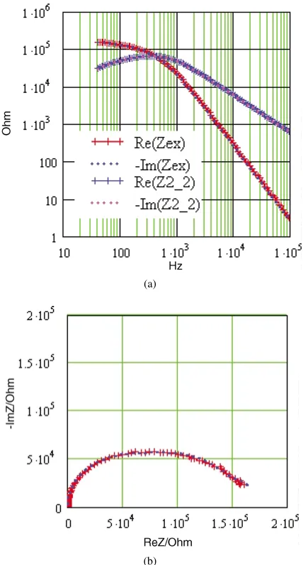
mea-sured by Agilent 4294A in the frequency range of 40 Hz–100 kHz. A fitting of the results to 2nd order 2nd family is presented in Fig. 4(a) (both the real and imagi-nary parts vs. frequency) and (b) (Cole-Cole plot). Note that the lines in those figures are doubled, as the experi-mental and fitting lines are very close. One could be eas-ily convinced that this is a good approximation. How-ever, looking at Fig. 5, one can see immediately that the new approach identifies it correctly as 4th order 1st fam-ily. Using the correct system function, ZView (Scribner Associates, Inc.) yields the following values after fit-ting with unit weighfit-ting: C0=1.14µF, C1=49.9 nF,

R1 =39.0 k, C2 = 4.01 nF, R2 = 67.6 k, C3 =

10.0 nF, R3=56.2 k.

Discussion and Summary

Partitioning of all the possible circuit models was de-veloped, based on increased complexity. Each system function represents a group of possible circuit mod-els, and is defined by its order and family. The order of the system function is the rank of the denomina-tor polynomial, and is also the number of capacidenomina-tors in the corresponding RC model circuits. There are but four different families of system functions describing all the possible RC circuits.

(a) (b)

(c) (d)

(e)

(a)

(b)

Fig. 4. Experimental data generated using circuit belongs to 4th order 1st family system function, compared with fitting using 2nd order 2nd family system function. (a) Real and imaginary data; (b) Cole-Cole plot.

consisting of R and C elements. If the spectrum can be modeled by nontrivial circuit elements like Warburg-or Gerischer-impedances (Warburg-or other transmission line models) application of the method would lead to high order RC model. In these cases, the usefulness of the method is limited to finding the minimum discrepancy that could be achieved. This, however, is an important piece of information, as it gives the experimentalist an un-biased criterion to evaluate any model by comparing the discrepancy it yields with the minimal discrepancy found for orders after the kink.

Fig. 5. Discrepancy vs. order for the experimental data of Fig. 4, showing that the best choice of system function is 4th order 1st family.

Recently, Schichlein et al. [7, 8] further developed a deconvolution approach [9] based on Fourier trans-form of the data. The authors pre-assume that a single cell SOFC belongs to what we call here 2nd family. The main advantage of the Schichlein et al. approach is that it allows one to find distribution of time con-stants within family 2, i.e., to deal with constant phase elements for instance. We believe that our approach can be combined with this and similar deconvolution approaches [10, 11] as a first step. Using our approach first, will give information on what the family is, how many time constants (or peaks in the time constant dis-tribution function) should be found and what is the discrepancy that one should expect from a good model for the present data. This, in turn, can provide a use-ful starting point to construct a proper regularization method for the ill-defined inverse problem of finding the time constant distribution function [12].

Acknowledgments

The authors gratefully acknowledge the financial sup-port of the Israel Science Foundation (grant no. 107/01-12.6), the Center for Absorption in Science—Ministry of Immigrant Absorption and the Technion’s Catalysis Center.

References

2. J.R. Macdonald and J.A. Garber,J. Electrochem. Soc.,124, 1022 (1977).

3. J.R. Macdonald, J. Schoonman, and A.P. Lehnen,J. Electroanal. Chem.,131, 77 (1982).

4. H.A. Kramers,Physik. Z.,30, 52 (1929). 5. R. de L. Kronig,J. Opt. Soc. Am.,12, 547 (1926).

6. L. Ljung,System Identification—Theory for the User (Prentice-Hall, 1987), Ch. 7.

7. H. Schichlein, M. Feuerstein, A. M¨uller, A. Weber, A.Kr¨ugel, and E. Ivers-Tiff´ee, inSolid Oxide Fuel Cells VI(Electrochem. Soc. Proc. Ser., 1999), p. 1069.

8. H. Schichlein, A. M¨uller, M. Voigts, A. Kr¨ugel, and E. Ivers-Tiff´ee,J. Appl. Electrochemistry,32, 875 (2002).

9. R.M. Fuoss and J.G. Kirkwood,J. Am. Chem. Soc.,63, 385 (1941).

10. F. Alvarez, A. Alegr´ıa, and J. Colmenero,J. Chem. Phys.,103, 798 (1995).

11. E. Tuncer and S.M. Guba´nski,IEEE Transctions on Dielectric and Electrical Insulation,8, 310 (2001).

12. W.H. Press, S.A. Teukolsky, W.T. Vetterling, and B.P. Flannery,