Viscous effects on wave generation by strong winds

doi:10.1017/S0022112007009858 Printed in the United Kingdom

Viscous effects on wave generation

by strong winds

A. Z E I S E L, M. S T I A S S N I E,A N D Y. A G N O N

Department of Civil and Environmental Engineering, Technion – Israel Institute of Technology, Haifa 32000, Israel

(Received17 April 2007 and in revised form 28 October 2007)

This paper deals with the stability of water waves in a shear flow. Both temporal and spatial growth rates are derived. A carefully designed numerical solver enables us to extend the range of previous calculations, and to obtain results for larger wavelengths (up to 20 cm) and stronger winds (up to a friction-velocity of 1 m s−1_). The main finding is the appearance of a second unstable mode which often turns out to be the dominant one. A comparison between results from the viscous model (Orr–Sommerfeld equations) and those of the inviscid model (Rayleigh equations), for 18 cm long waves, reveals some similarity in the structure of the eigenfunctions, but a significant difference in the imaginary part of the eigenvalues (i.e. the growth rate). It is found that the growth rate for the viscous model is 10 fold larger than that of the inviscid one.

1. Introduction

1.1. Background and motivation

The discussion of wave generation in modern science is almost 150 years old, since the days of Kelvin, Stokes, Rayleigh and others. The history of scientific publications on the subject in the 20th century began when Jeffreys (1925) published his sheltering theory. Major progress was made with the publication of two groundbreaking studies by Miles (1957a) and by Phillips (1957). These two studies suggest two different mechanisms for wave generation. Phillips argued that waves can be generated by a resonance mechanism between the air turbulent eddies and the water. He assumed that the water is an inviscid fluid and the initial water state is rest. Miles proposed that the growth of waves is caused by interaction of the surface waves with a parallel shear flow. He assumed that the fluids are inviscid and presented Rayleigh’s equation as the governing equation of the problem. In recent years, it has become clear that the shorter waves (with a wavelength less than say 20 cm), which contain only a small fraction of the total energy-density, play a significant role in the overall dynamics. For these waves we must include surface tension as well as viscous effects in the analysis. The growth of these shorter waves, under the influence of rather strong winds, is the focus of this paper.

1.2. Theoretical and numerical references

1.3. Experimental references

Larson & Wright (1974) provide a comprehensive experimental study of the temporal growth of gravity–capillary waves. They use microwave backscatter as a measurement technique. Larson & Wright find that the growth rate is independent of the fetch, dependent on the wavenumber and varies with u_∗ like a power law. Caulliez, Ricci & Dupont (1998) study experimentally the first visible ripples that appear on the water surface. They argue that the laminar–turbulent transition of the near-surface water flow causes an explosive growth of the wind-generated ripples. As previously mentioned, Tsaiet al.(2005), also perform experimental studies of the spatial growth of gravity–capillary waves. They measure a laminar wind profile at varying fetches and emphasize the development of the boundary layer with fetch. In all these papers, the subject of the wind velocity profile is a dominant issue and a variety of profiles is used.

1.4. Wind profile studies

Charnock (1955) measures the air mean velocity profile above a large reservoir. He finds that the air flow fits a logarithmic law. Miles (1957b) suggests an approximation to the solution of the boundary-layer equation which has a linear zone and a logarithmic-like profile. Many authors find this profile useful because of its smooth first derivative for all values of u_∗ and matching height between the linear and the logarithmic regions. Most of the field measurements were conducted at low wind speeds. As evidence of the nature of air flow above water at high-speed wind, we can cite Powell, Vickery & Rienhold (2003) who made field measurements in tropical cyclones. They found that the wind profile correlates very well with the logarithmic shape in the first 200 m.

2. Mathematical formulation

2.1. Linear stability model

The starting point is the governing equations for an incompressible viscous fluid flow, which are the Navier–Stokes and continuity equations.

ˆ

ρ

∂V

∂t +V· ∇V

=−∇P +µ∇2V +gρ,ˆ (2.1)

∇ ·V = 0. (2.2)

We write the velocity and the pressure fields as:

V = (U(z) +u(x, z, t), v(x, z, t)), (2.3)

P =p0−ρgzˆ +p(x, z, t). (2.4)

Where U(z) is the mean flow profile, u, v and p are harmonic perturbations of the horizontal velocity, vertical velocity, and pressure, respectively; in the above equations

x and z are the horizontal and vertical coordinates, respectively, and t is the time;

g,µ,ˆ ρˆ are the acceleration due to gravity, dynamic viscosity and density, respectively. We can separate the equations into harmonic terms and steady terms, and apply the assumption that the perturbations are infinitesimal, in order to linearize them. Since we are looking for a solution which has a harmonic part and a vertical dependent part, we write:

u= ˜u(z)ei(kx−ωt)_{, v= ˜v(z)e}i(kx−ωt)_{, p= ˜p(z)e}i(kx−ωt)_{, η=η}

Where ω, k, η are the wave frequency, wavenumber and interface elevation, respectively. We can define a perturbation streamfunction which has the form:

ψ =f(z)ei(kx−ωt), (2.6)

where f(z) is the auxiliary function, and the relations between the streamfunction and the velocity components give:

˜

v=−ikf(z), ˜u=f(z). (2.7)

The prime denotes vertical differentiation. After a simple elimination process, we find that the governing ODE forf(z) is the Orr–Sommerfeld equation:

iν(f(4)−2k2f+k4f) +k(U−c)(f−k2f)−Uf= 0, (2.8)

where ν and c are the kinematic viscosity and the phase velocity, respectively. The domains of the air and water are assumed to be semi-infinite, and we have boundary conditions at positive or negative infinity and at the interface between the fluids. At infinity, the perturbations are assumed to decay exponentially. At the interface, we impose the kinematic boundary condition, horizontal velocity continuity, shear stress continuity and the dynamic boundary condition (continuity of normal stress). All of the boundary conditions are imposed atz= 0, after the linearization procedure. For the full formulation of the boundary conditions see Valenzuela (1976). We choose the reference problem of linear water waves without wind and current, neglecting the influence of the air, for which the wavenumber and the wave frequency are related by:

ω2₀ =gk0+

σ k3

0

ρw

, (2.9)

where σ is the surface tension. Transforming to dimensionless quantities (note that the circumflex in (2.10) denotes a dimensional quantity):

ω= ωˆ

ω0

, k= kˆ

k0

, c= cˆ

c0

,

z= ˆzk0, U=

ˆ

U

c0

, f = f kˆ 0

η0ω0

.

(2.10)

Defining the dimensionless numbers of the problem:

Rw,a=

c0

νw,ak0

, F = 1

F2

r = gk0

ω2

0

, W = 1

We

= σ k 3 0

ρwω2₀

, ρ= ρa

ρw

, µ= µa

µw

, (2.11)

whereR is the Reynolds number,F is the inverse square Froude number, W is the inverse Weber number, ρ is the density ratio and µ is the dynamic viscosity ratio. The subscriptswand a refer to water and air, respectively. The complete eigenvalue problem must satisfy the following system:

Two ODEs:

iR−1w

fw(4)−2k2fw+k4fw

Viscous terms

+k(Uw−c)

fw−k2fw

−Uwfw

= 0, z∈(−∞,0],

(2.12) iR_a−1f_a(4)−2k2f_a+k4fa

Viscous terms

+k(Ua−c)

f_a−k2fa

−U_afa

Nine boundary conditions:

fa(0) =c−U(0), fw(0) =c−U(0), (2.14)

f_w +U_w =f_a+U_a atz= 0, (2.15)

µ(f_a+k2fa+Ua) = (fw+k 2_f

w+Uw) atz= 0, (2.16)

kf_w(c−U0) +kfwUw + iR−

1 w

3k2f_w −f_w

Viscous terms

−kF

=ρ

⎡ ⎢

⎣kfa(c−U0) +kfaUa+ iRa−1

3k2fa−fa

Viscous terms

−kF

⎤ ⎥

⎦+W k3 atz= 0, (2.17)

fw(z)→0, fw(z)→0, z→ −∞, (2.18)

fa(z)→0, fa(z)→0, z→ ∞. (2.19) When formulating the inviscid model, we neglect the viscous terms in (2.12) and (2.13) and obtain two Rayleigh equations. The boundary conditions will be the kinematic boundary condition in the same form (2.14), and the dynamic boundary condition without the viscous terms (2.17). Conditions (2.15) and (2.16) do not apply when formulating the inviscid case. Both the viscous and inviscid models are classified as eigenvalue problems. The calculations will focus on the temporal and spatial cases, meaning that the growth can be only either in space, or in time. For the temporal case we specifyk and search forω, and for the spatial case we specify ω and search for k.

2.2. Mean flow profile

In (2.12) to (2.19), U(z) represents the mean flow profile. It is already well known (Kawai 1979; Van Gastel et al. 1985; Wheless & Csanady 1993), that the results are sensitive to the profile shape. The exact mean flow profile above water waves is still uncertain. Miles (1957b) suggests a profile which fits well the mean flow profile above a flat plate. This profile was used in previous studies Valenzuela 1976; Kawai 1979; Van Gastel et al. 1985), and was named the ‘lin–log’ profile. We use this profile for the air, and an exponential profile for the current in the water.

In the air (wind profile):

Ua =

⎧ ⎪ ⎨ ⎪ ⎩

U0+

u2

∗

νa

z, z6z1,

U0+mu∗+ u_κ∗

α−tanh

_α 2

, z>z1,

(2.20)

and in the water (current profile):

Uw=U0exp

ρau2_∗

U0µw

z

(2.21)

where,

α= sinh−1(β), β= 2κu∗

νa

(z−z1), z1=

mνa

u_∗ , U0=Bu∗, m= 5, B= 0.5, (2.22)

0 2 4 6 –2

0 2 4 6 8 10

Ua(m s–1) Ua(s–1) Ua(m–1 s–1)

z

(m)

(a)

0 5000 10000 15000

(b)

–10 –5 0

(c)

u_{* = 0.1} (m s–1)

u_{* = 0.3} (m s–1₎

u_{* = 0.5} (m s–1₎

(×107)

(×10–4)

–2 0 2 4 6 8 10

(×10–4)

–2 0 2 4 6 8 10

(×10–4)

Figure 1.The base flow and its first two derivatives for the linear–logarithmic profile and

various values of u_∗(m= 5). (a) The velocity profile, (b) the first derivative, (c) the second

derivative.

m in (2.22) defines the thickness of the viscous sublayer (the linear segment), and thus influences the derivative at the interface. This profile enables continuity of the function and its first two derivatives at the matching pointz=z1 for all values of the parametersmandU0. The value ofmis set to 5 (usuallym= 5−8), whereas the value ofB is chosen to beB= 0.5 according to Kawai (1979), this value can sometimes be taken asB= 0.3 as found by Zhang & Harrison (2004), but qualitatively it would not change the results. The value of B controls the drift current, but also influences the derivatives of the current. This profile, in (2.20) and (2.21), maintains the continuity of the shear stress between the air and the water,µaUa=µwUw.

As can be seen in figure 1, the friction velocity u_∗ defines the wind intensity as well as the current profile. The first and second derivatives have discontinuities at the interface, but are continuous in the air. The first two derivatives have increasing absolute values asu_∗ increases.

2.3. Alternative wind profile

As an alternative wind profile, we present a wind profile which will enable us to compare the inviscid and viscous solutions under strong winds. This profile is based on the numerical solution of the turbulent boundary-layer equation, which is:

µa

dU

dz

Laminar stress

+ρaκ2z2

dU

dz

2

Turbulent stress

=τ0=ρau2_∗. (2.23)

(×107)

0 2 4

–2 0 2 4 6 8 10

Ua(m s–1) Ua(s–1) Ua(m–1 s–1)

z

(m)

(a)

0 5000 10000 15000

(b)

–10 –5 0

(c)

u_{* = 0.1} (m s–1)

u_{* = 0.3} (m s–1₎

u_{* = 0.5} (m s–1₎

(×10–4)

–2 0 2 4 6 8 10

(×10–4)

–2 0 2 4 6 8 10

(×10–4)

Figure 2. The base flow and its first two derivatives from the numerical integration of the

boundary-layer equation for various values ofu_∗. (a) The velocity profile, (b) the first derivative,

(c) the second derivative.

§2.2. The benefit from this kind of profile is that it enables to compare the viscous and inviscid solutions at any wind intensity. We named this profile the ‘numerical’ profile. The profile and its derivatives are described in figure 2; it is very similar to the lin–log profile, but with a much thinner viscous sublayer.

3. Numerical procedure and its validation

3.1. Numerical procedure

The numerical procedure which we used to solve the eigenvalue problem of the viscous model is based on the Chebyshev collocation method. We chose this method because of the difficulties in the integration of the Orr–Sommerfeld equation, which forced some of the previous authors to use filters in order to remove parasitic errors. Another reason for this choice is the nature of the Chebyshev grid which is characterized by a high density of grid points near the boundaries. The Chebyshev grid is:

xj = cos

jπ

N

∀j = 0,1, . . . , N . (3.1)

The method approximates an unknown function by a finite series of Chebyshev polynomials see (Trefethen 2000).

φ(x) =

N

n=0

anTn(x). (3.2)

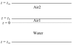
Air2

Air1

Water

z = z_∞

z = z_∞ z = z1

z = 0

Figure 3.Computational domain of the problem.

means thatzdimensional,_±∞≈ ±1.6λ, whereλ= 2π/k0 is the reference wavelength. The lower interval is for the water, the upper layer (air2) is for the logarithmic air region, and the intermediate interval (air1) is for the viscous sublayer region (see figure 3). Linear transformations are used to transform each interval into [−1,1], which is where the Chebyshev polynomials are orthogonal.

Since the problem at hand is an eigenvalue problem, we search for a pairω, kwhich causes the solution to obey all 9 boundary conditions. An iterative process to find this eigenvalue was built. This process begins with an initial guess for the eigenvalue; the next stage is to solve the coupled BVP (boundary value problem) and finally to use a standard secant method to produce an improved guess. The process is stopped when a convergence condition, requiring four significant digits in the imaginary part of the eigenvalue, is satisfied. The Chebyshev collocation method is used for the solution of the BVP. This search process provides only one eigenvalue at a time; the specific eigenvalue which the process converges to depends on the initial guess. This approach is different from the one of solving the generalized eigenvalue problem and finding all of the eigenvalues, see Boomkampet al.(1997).

In practice, we reduce the order of the Orr–Sommerfeld equation by defining

V ,f and replacing the Orr–Sommerfeld equation with the system:

V −f= 0, (3.3a)

iR−1(V−2k2V +k4fa) +k(Ua−c)(V −k2fa)−Uafa

= 0. (3.3b) The next step is to transform the differential equations into an algebraic form with the help of the Chebyshev differentiation matrices. We solved the BVP with all of the boundary conditions, except for the dynamic boundary condition (2.17). In practice we, add an artificial interface between the air1 domain and the air2 domain, and actually solve three coupled Orr–Sommerfeld equations. The boundary conditions between air1 and air2 are similar to the boundary conditions between the water and air in their physical meaning; but since the density, viscosity and the base flow are continuous, they are written as:

fa2(z1) =fa1(z1), fa2(z1) =fa1(z1), fa2(z1) =fa1(z1), fa2(z1) =fa1(z1). (3.4)

The iterative process is built for the functionG(ω, k), which is defined as:

G(k, ω) =kfw(c−U0) +kfwUw +iR−

1 w (3k

2

fw −fw)−kF

−ρkfa(c−U0) +kfaUa+iRa−1(3k2fa−fa)−kF

−W k3 at z= 0. (3.5)

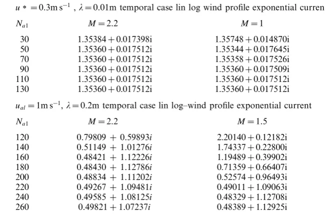
u∗= 0.3m s−1 _{,λ= 0.01m temporal case lin log wind profile exponential current}

Na1 M= 2.2 M= 1

30 1.35384 + 0.017398i 1.35748 + 0.014870i

50 1.35360 + 0.017512i 1.35344 + 0.017645i

70 1.35360 + 0.017512i 1.35358 + 0.017526i

90 1.35360 + 0.017512i 1.35360 + 0.017509i

110 1.35360 + 0.017512i 1.35360 + 0.017512i

130 1.35360 + 0.017512i 1.35360 + 0.017512i

ual= 1m s−1,λ= 0.2m temporal case lin log–wind profile exponential current

Na1 M= 2.2 M= 1.5

120 0.79809 + 0.59893i 2.20140 + 0.12182i

140 0.51149 + 1.01276i 1.74337 + 0.22800i

160 0.48421 + 1.12226i 1.19489 + 0.39902i

180 0.48430 + 1.12786i 0.71359 + 0.66407i

200 0.48834 + 1.11202i 0.52574 + 0.96493i

220 0.49267 + 1.09481i 0.49011 + 1.09063i

240 0.49585 + 1.08125i 0.48329 + 1.12708i

260 0.49821 + 1.07237i 0.48389 + 1.12925i

Table 1. Convergence of the Chebyshev collocation method for two wind intensities and

wavelengths, temporal case. WhereNa1=Nw, Na2=MNa1. (Values ofω.)

property of the BVP, and, to a certain extent, it defines the distance between a chosen solution of the BVP and that of the eigenvalue problem. Note that all the results in this paper were calculated using the following numerical values:

κ= 0.41, µw= 10−3pa s, µa = 1.83 10−5pa s,

ρa = 1.225kgm−3, ρw= 1000kg m−3, g = 9.81ms−2, σ = 0.075N m−1

(3.6)

3.2. Validation of the numerical results

In this section we will show the convergence of the Chebyshev collocation method, test the sensitivity of the model to the interval size and compare the results with a test case and previous studies. An analytical solution for the viscous problem with a linear wind profile and a constant current is given in the Appendix, and serves as the test case.

3.2.1. Convergence of the Chebyshev collocation method

As mentioned above, the computational domain is divided into three sub intervals: the water [−z_∞,0], the air1 [0, z1] and the air2 interval [z1, z∞]. In each of these intervals we can control the number of collocation points (the grid). If the method converges, the change in the results should be minor when changing the number of collocation points. From numerical experiments, we learn that the interval air1 is the most important interval and therefore requires a high resolution grid. We show convergence, for the case where the number of collocation points in the interval air1

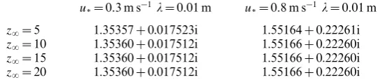
u_∗= 0.3 m s−1 _{λ= 0.01 m u}

∗= 0.8 m s−1 λ= 0.01 m

z_∞= 5 1.35357 + 0.017523i 1.55164 + 0.22261i

z_∞= 10 1.35360 + 0.017512i 1.55166 + 0.22260i

z_∞= 15 1.35360 + 0.017512i 1.55166 + 0.22260i

z_∞= 20 1.35360 + 0.017512i 1.55166 + 0.22260i

Table 2. The sensitivity ofωto differentz_∞, temporal case, lin–log wind profile, exponential

current.

Temporal case

λ= 0.001m λ= 0.1m λ= 0.2m

u_∗= 0.001 m s−1 _{Numerical 1.0705−0.017431i 1.1246 + 0.0071116i 1.0908 + 0.0091061i}

Analytical 1.0705−0.017431i 1.1246 + 0.0071115i 1.0908 + 0.0091070i

u_∗= 0.005 m s−1 _{Numerical 1.3628−0.016102i 1.7260 + 2.2254i 1.7684 + 2.5485i}

Analytical 1.3628−0.016102i 1.7262 + 2.2254i 1.7680 + 2.5489i

u_∗= 1 m s−1 _{Numerical 1.7132−0.000028672i 0.47194−7.6548i 5.3226 + 8.4767i}

Analytical 1.7132−0.000029147i 0.46973−7.6153i 5.3219 + 8.4752i

Table 3.Comparison with test case, temporal case for various wind intensities and

wavelength. (Values ofω.)

3.2.2. Sensitivity toz_∞

Since, in practice, we need to use a finite interval for the numerical calculations, we must show that our choice does not have a major effect on the results. The z

coordinate is normalized by k0 in the form z=zdimensionalk0. From a physical aspect, the value of z_∞ should be related to the wavelength. From linear theory of water waves, it is known that at depths below half a wavelength, the influence of the waves on the flow field is minor. The value which we use for most of our calculations is

z_∞= 10, which means that z_∞,dimensional= 10λ/(2π) = 1.591λ. In order to justify this value, we made a few runs with different values ofz_∞. Note that in this method, when we change the interval size we need to change the number of collocation points in order to keep a fine grid in the critical region. From table 2 we can state that if there is an error it is in the fourth digit.

3.2.3. Comparison with the test case

In order to validate the numerical results, we want to compare them with an analytical solution. The case which we compare them with is the one mentioned at the beginning of§3.2. The analytical solution of this case is based on a combination of Airy and exponential functions, thus the numerical solution is not so trivial, for details see Appendix. Such a comparison has significant meaning, because the methods which were used to obtain the results are completely different from each other. The comparison was made for the spatial case, as well as for the temporal case. The current was constant with the value ofUw= 0.5u∗ and the velocity slope of the wind wasu_∗/νa. These conditions are similar to those which were used in the lin-log profile. The results are described in table 3. The maximum error in this comparison is 2%, whereas in most of the cases the error is smaller than 1%.

3.2.4. Comparison with previous studies

1 3 5 7 9 0

1 2 3

k (cm–1₎

2

β

(s

–1)

u_* = 0.13 m s–1

u_* = 0.17 m s–1

u_* = 0.214 m s–1

u_* = 0.248 m s–1

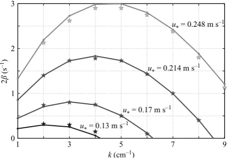
Figure 4. Energy growth rate vs. wavenumber, temporal case. Comparison with previous

studies. Solid line, our study; five point star, results from Tsai & Lin (2004), (analogous to figure 2 in Tsai & Lin 2004).

They all compute similar values for the temporal growth rate, but for a rather small domain in the (λ, u_∗)-plane. Figure 4 is analogous to figure 2 in Tsai & Lin (2004).

In figure 4, there are symbols of our calculations and symbols of Tsai & Lin’s calculations taken from figure 2 in Tsai & Lin (2004). We can see that the results of Tsai & Lin (2004) are similar to our results; the difference is up to 5%, but is typically of the order of 1%. For the spatial case, we are not familiar with previous studies to which it may be compared. Finally, it seems safe to say that for the range of λ ∈ (0.001,0.2) m, u_∗ ∈ (0,1) m s−1_{, our numerical results are reliable. In most} cases, accuracy is to the first four digits, whereas in the more difficult cases it is only to the first two significant digits.

4. A second eigenvalue at high wind intensities

4.1. Results for the temporal case

A number of studies concerning the surface wave stability problem have been conducted (e.g. Valenzuela 1976; Tsai et al. 2005 and references therein). All of the results that we found were limited in wind intensity and in wavelength/wave period. Most of the theoretical studies focus on the temporal case, except for Tsai et al. (2005) which deals with spatial evolution for a laminar base flow. The domain of previous calculations in the range of approximately, wavelength 0<λ<7 cm, and friction velocities 0< u_∗<0.5 m s−1_{, is plotted in figure 5. As described in §3.2, our} solver for the viscous problem is valid in the domain 0<λ<20cm,0< u_∗<1m/sec

0.04 0.08 0.12 0.16 0.20 0

0.2 0.4 0.6 0.8 1.0

λ = 0.04 m λ = 0.12 m _λ = 0.18 m

u_* = 0.3 m s–1

u_* = 0.6 m s–1

u_* = 0.8 m s–1

Previous studies

One unstable mode Two unstable modes

Rayleigh's equation does not produces growth u*

(m s

–1

)

λ (m)

Figure 5.Instability domains of the solution over the (λ, u_∗)-plane. solid line, boundary of

the region where there are two unstable modes; solid thin line- neutral line (zero growth rate); dash-dot line, the domain of previous studies; dashed line, the region where the inviscid model produces growth. Temporal case, the profile is according to (2.20)–(2.22).

0.2 0.4 0.6 0.8 1.0

0 1

(a)

Im (ω)

——–_ω

0

u_* (m s–1)

0.2 0.4 0.6 0.8 1.0

0 1

(b)

0.2 0.4 0.6 0.8 1.0

0 1

(c)

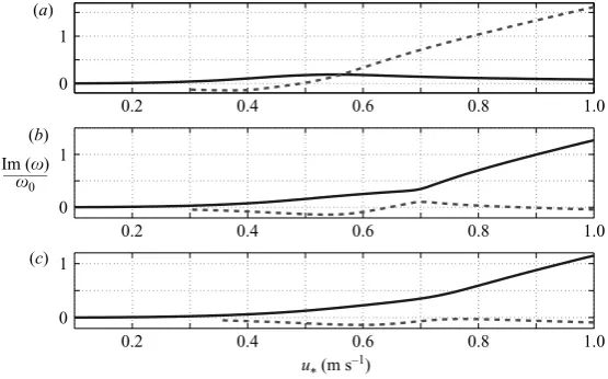
Figure 6.Normalized imaginary part of the frequency vs. friction velocity for various

wavelengths, two modes are shown in the region of interest, temporal case, the profile is

according to (2.20)–(2.22). (a)λ= 0.04 m, (b)λ= 0.12 m, (c)λ= 0.18 m. The solid line and the

dashed line are two distinct solutions for the specific scenario.

0.2 0.4 0.6 0.8 1.0 2.0

1.0

(a)

Re (ω)

——–_ω

0

u_* (m s–1)

0.2 0.4 0.6 0.8 1.0

0.5 1.0

0.5 1.0

(b)

0.2 0.4 0.6 0.8 1.0

(c)

Figure 7. Normalized real part of the frequency vs. friction velocity for various wavelengths,

two modes are shown in the region of interest, temporal case, the profile is according to

(2.20)–(2.22). (a)λ= 0.04 m, (b) λ= 0.12 m, (c) λ= 0.18 m. The solid line and the dashed line

are two distinct solutions for the specific scenario.

0.04 0.08 0.12 0.16 0.20

1.0

0.5

0 0

0.04 0.08 0.12 0.16 0.20

0

0.04 0.08 0.12 0.16 0.20

0

(a)

Im (ω)

——–_ω

0

λ(m )

0 0.2

–0.2

–0.02 0.4

0.06

0.02 0

(b)

(c)

Figure 8. Normalized imaginary part of the frequency vs. wavelength for various friction

velocities, two modes are shown in the region of interest, temporal case, the profile is according

to (2.20)–(2.22). (a)u_∗= 0.8 m s−1_{, (b)u}

∗= 0.6 m s−1, (c)u∗= 0.3 m s−1. The solid line and the

dashed line are two distinct solutions for the specific scenario.

0.04 0.08 0.12 0.16 0.20 1.5

1.0

0.5

1.5

1.0

0.5

1.4

1.2

1.0 0

0.04 0.08 0.12 0.16 0.20

0

0.04 0.08 0.12 0.16 0.20

0

(a)

Re (ω)

——–_ω

0

λ(m )

(b)

(c)

Figure 9.Normalized real part of the frequencyvs. wavelength for various friction velocities,

two modes are shown in the region of interest, profile is according to (2.20)–(2.22). (a)

u∗= 0.8 m s−1_{, (b)u}

∗= 0.6 m s−1_{, (c)u}

∗= 0.3 m s−1_{. The solid line and the dashed line are two}

distinct solutions for the specific scenario.

0.04 0.08 0.12 0.16 0.20

0 40 80 120 160

λ (m)

Im (

ω

) (s

–1)

Figure 10.Temporal growth rate vs. wavelength, _u∗= 1 m s−1, the profile is according to

(2.20)–(2.22). The solid line and the dashed line are two distinct solutions for the specific scenario.

0 5 10 –1.0

–0.8 –0.6 –0.4 –0.2 0 0.2 0.4 0.6 0.8 1.0

|f |/η0 (m s–1)

z

(m)

(a) (b) (c)

1 2 3

arg( f )

0 5 10 15

ρ(u2 _{+ v}2_)/2η 0

2 _{(kg m}–2 _s–2_{) (×10}8₎

branch1 ω = 1.17 + 0.14i critical point branch2 ω = 0.43 + 0.71i critical point

z1

–1.0 –0.8 –0.6 –0.4 –0.2 0 0.2 0.4 0.6 0.8 1.0

z1

–1.0 –0.8 –0.6 –0.4 –0.2 0 0.2 0.4 0.6 0.8 1.0

z1

(×10–3) (×10–3) (×10–3)

Figure 11. Comparison of the vertical structure of the eigenfunction and the kinetic energy

density between the two modes forλ= 0.04 m, u∗= 0.7 m s−1_{, temporal case, profile is according}

to (2.20)–(2.22). (a) absolute value of the eigenfunction, (b) argument of the eigenfunction, (c) kinetic energy density.

produce growth for longer wavelengths. The results for both, the point of maximum growth and the neutral point, are very intuitive and show that: when increasing the wind intensity, the value of maximum growth becomes larger and the wavelengths of maximum growth and zero growth become shorter. The real part of the eigenvalue, described in figure 9, shows a major difference between these two branches of the solution. While one of the branches has a phase velocity which is often higher than the reference case, (Re(ω)/ω0>1), the second branch has a phase velocity which is lower than the reference case, (Re(ω)/ω0<1). The result that the phase velocity of the wave usually decreases when the friction velocity increases is not very intuitive. This result was also obtained by Valenzuela (1976).

In figure 10 the temporal growth rate is presented in dimensional form. As we can see, the values of the growth rate are very large, especially for waves in the gravity– capillary range. These ‘explosive’ growth rates which can exist in very strong winds (u_∗= 1 m s−1_{, i.e. U}

10= 37 m s−1), indicate that these ripples attain their maximum steepness almost immediately, and break continuously.

While comparing the eigenfunctions of both modes in figure 11, we can see a significant similarity in the air region, but a profound difference in the water region. The horizontal dashed line in this figure indicates the edge of the laminar layer, and it is clear that most of the energy transfer from the mean flow to the disturbance happens within this layer. The square and circle symbols indicate the location of the so-called critical point, where the mean flow velocity is equal to the actual phase velocity. We can see that the critical-points, for both modes, are in the water and that they do not play any significant role in the case at hand.

can state that the second unstable mode appears only when the mean flow profile includes a shear current. Another condition is that the wind intensity will be above a critical value. The results in the figures were calculated for a specific lin–log profile (m= 5, B= 0.5 see (2.22)), the parameter B which controls the drift current has a major influence on the critical conditions for the appearance of the second mode. In order to identify the conditions that influence the appearance of the second unstable mode, we have tried many combinations of wind profiles/intensities and current profile/intensities. In figure 12, we present six dynamic boundary condition plots, (see definition in §3.1) that demonstrate the behaviour of the problem for different scenarios. The left-hand column is for a relatively low wind intensity (u_∗= 0.3 m s−1), and the right-hand column is for a high wind intensity (u_∗= 0.8 m s−1), whereas the three different rows are for current only (no wind), wind with constant current (no shear in the water), and wind with exponential current; from top to bottom, respectively. From figures 12(a) and 12(d), we can see that the exponential current by itself can cause instability, but does not cause two unstable modes. From figures 12(b) and 12(e), we can conclude that a current without shear can not cause two unstable modes. In figures 12(c) and 12(f), we can see that for the combination of the wind and current the picture looks very different, particularly at strong winds, where the two unstable modes appear.

As already mentioned, the physical reason for the appearance of the second growing eigenvalue is not entirely clear. However, the fact that its phase velocity is smaller than c0 (sometimes much smaller), and that it appears only above a threshold ofu∗, which corresponds to a threshold in the drift-current, provides some indication that the second eigenvalue originates from a left moving wave which evolved into a right moving wave under the influence of the current. To check if this assumption makes sense, we refer to figure 13 where we compare the solid-line separating the domains of one and two solutions with two approximated theoretical lines. An approximation for the lower boundary of the solid line can be obtained by a simple equation (dashed line) which states the equality of the drift velocity and the unperturbed phase velocity:

1

2u∗ =c0. (4.1)

Note that (4.1) is motivated by the case of a constant (i.e. a zindependent) current. To attain an approximation for the upper boundary, which separates the domains of one and two solutions, we have to consider the fact that the current varies with depth, and compare its vertical decay rate with that of the disturbance. From (2.21), we see that the decay rate of the current is (2ρau∗)/µw, whereas the vertical decay rate of the wave is given byk0; comparing the two yields:

2ρau_∗

µw

=αk0, (4.2)

where α is a somewhat free dimensionless constant. Note that the dash-dot line in figure 13 is plotted withα= 30, this value was chosen to obtain a fit atu_∗= 1 m s−1_.

4.2. Results for the spatial case

0.02 0.03 0.04 0.05

0.060.07 _0.0

8 0.09 0.1 0.1₁ 0.12 0.13 0.13

0.14 0.14 0.15

0.15 0.16

0.16

0.17 _0.1

7

0.18 0.18

0.19 0.19 0.2 0.2 0.3 0.3 0.5 0.5 0.5 0. 7 0.7 0.7 0.7 0.9 0.9 0.9 0.9 0.9 1.1 1.1 1.1 1.1 1.₃ 1.3 1.3 1.3 1.5 1.5 1.5 1.5 1.7 1.7 1.7 1.7 1.9 1.9 1.9 1.9 2.1 2.1 2.1 2.1 2.3 2.3 2.3 2.3 2.5 2.5 2.5 2.5 2.7 2.7 2.7 2.7 2.9 2.9 2.9 2.9 3.1 3.1 3.1 3.1 3.3 _3.3 3.3 3.3 3.5 _3.5 3.5 3.5 3.7 _3.7 3.7 3.7 3.9 _3.9 3.9 3.9 4.1 4.1 4.1 4.3 4.3 4.5 4.5 4.7 4.7 4.9 4.9 5.1 5.1 5.3 5.3 5.5 5.5 5.7_5.96.1 6.36.5 6.77.17.37.57.7_6.9

7.98.18.38.58.7

ωi

—

ω0

0.4 0.6 0.8 1.0 1.2 1.4 1.6

0.2 0.4 0.6 0.8

1.14 – 0.005i

(a)

0.01 0.02 0.03 0.04 0.0_50.06 0.070.08

0.00.1₉

0.1 0.11 0.11 0.1 2 0.12 0. 13 0.13 0.1₄ 0.14 0.15 0.15 0.16 0.16 0.1₇ 0.17 0.1₈ 0.18 0.19 0.1₉ 0. 2 0. 2 0.3 0.3 0.3 0.5 0.5

0.5 0.5

0.7 0.7

0.7 0.7 0.7 0.9 0.9 0.9 0.9 1.1 1.1 1.1 1. 1 1.3 1.3 1.3 1. 3 1.3 1.5 1.5 1.5 1.5 1.5 1.7 _1.7 1.7 1.7 1.7

1.9 1.9

1.9 1.9 1.9 2.1 2.1 2.1 2.1 2.1 2.3 2.3 2.3 2.3 2.3 2.5 2.5 2.5 2.5 2.5 2.7 2.7 2.7 2.7 2.7 2.9 2.9 2.9 2.9 2.9 3.1 3.1 3.1 3.1 3.1 3.3 3.3 3.3 3.3 3.3 3.5 3.5 3.5 3.5 3.5 3.7 3.7 3.7 3.7 3.7 3.9 3.9 3.9 3.9 3.9 4.1 4.1 4.1 4.1 4.1 4.3 4.3 4.3 4.3 4.3 4.5 4.5 4.5 4.5 4.5 4.7 4.7 4.7 4.7 4.7 4.9 4.9 4.9 4.9 5.1 5.1 5. 1 5.1 5.3 5.3 5.3 5.3 5.5 5.5 5.5 5.5 5.7 5.7 5.7 5.7 5.9 5.9 5.9 5.9 6.1 6.1 6.1 6.1 6.3 6.3 6.3 6.3 6.5 6.5 6.5 6.7 6.7 6.7 6.9 6.9 6.9 7.1 7.1 7.1 7.3 7.3 7.3 7.5 7.5 7.5 7.7 7.7 7.7 7.9 7.9 7.9 8.1 8.1 8.1 8.3 8.3 8.3 8.5 8.5 8.5 8.7 8.7 8.7 8.9 8.9 8.9 9.1 9.1 9.1 9.3 9.3 9.3 9.5 9.5 9.5 9.7 9.7 9.7 9.9 9.9 9.9 10 10 10 15 15 20

0.865 + 0.0508i

0.0030.005

0.007 0.00 9 0.02 0.03 0.04

0.05 0.06

0.07 0.07

0.

08

0. 08

0.09 0.09

0.1

0.1

0. 11

0.1₁

0.12 0.

12 0.1 3 0.₁₃ 0.14 0.14

0.150.1 0.15

6 0.1₆ 0.17 0.1₇ 0.18 0.1₈ 0.19 0.19 0.2 0.2 0.3 0.3 0.5 0.5 0.5 0.7 0.7 0.7 0.9 0.9 0.9 0.9 1.1 1.1 1.1 1.1 1.3 1.3 1.3 1.5 1.5 1.5 1.7 1.7 1.7 1.9 1.9 1.9

2.1 2.3 2.1 2.1

2.3 2.3 2.5 2.5 2.5 2.7 2.7 2.7 2.9 2.9 2.9 3.1 3.1 3.1 3.3 3.3 3.3 3.5 3.5 3.7

3.9 _4.14.34.54.7

1.448 + 0.0351i

0.02_0.03 0.04 0.050. 06 0.07 0.08 0.090.1 0.0.11012.13

0.14 0.15 0.16

0.17 0.18 0.19 0.2 0. 3 0.3 0.5 0.5 0.7 0.7 0. 9 0.9 0.9 1. 1 1.1 1.1 1.3 1.3 1.3 1.3 1.5 1. 5 1. 5 1.5 1.5 1.7 1. 7 1. 7 1.7 1.9 1.9 1.9 1.9 2.1 2. 1 2.1 2.3 2. 3 2.3 2.5 2.5 2.5 2.7 2.7 2.7 2.9 2.9 2.9 3.1 3.1 3.1 3.3 3.3 3.3 3.5 3.5 3.5 3.7 3.7 3.7 3.9 3.9 3.9 4.1 4.1 4.1 4.3 4.3 4.3 4.5 4.5 4.7 4.7 4.9 4.9 5.1 5.1 5.3 5.3 5.5 5.5 5.7 5.7 5.9 5.9 6.1 6.3 6.5 6.7 6.9 7.1 7.3 7.5 7.7 7.9 8.1

1.845 + 0.996i

0. 05 0.0₅ 0.05 0.1 0.1 0.1 0.1 0.15 0.15 0.15 0. 2 0.2 0.2 0. 25 0.25 0.25 0. 3 0.3 0. 3 0.3 0.35 0.35 0.₃₅ 0.35 0.4 0.4 0.4 0.4 0.4 0.4₅ 0.45 0.45 0.45 0.45 0.5 0. 5 0.5 0.5 0.5 0.6 0. 6 0. 6 0.6 0.6 0.7 0.7 0. 7 0.7 0.7 0.8 0.8 0.8 0.8 0.9 0.9 0.9 0.9 1 1 1 1 1 1.1 1. 1 1.1 1.1 1.2 1.2 1.2 1.2 1.3 1. 3 1.3 1.3 1.4 1. 4 1.4 1.4 1.5 1. 5 1.5 1.5 1.6 1.6 1.6 1.6 1.7 1.7 1.7 1.7 1.8 1.8 1.8 1.81.9 1.9 1.9 1.9 2 2 2 2 10 10 10 15

ωr/ω0

ωr/ω0

0.4 0.6 0.8 1.0 1.2 1.4 1.6 1.8 1.99

0 0.1 0.2 0.3 0.4 0.5 0.6 0.7 0.8 0.9 0.99

1.132 + 0.128i 0.5472 + 0.834i

0.05 0.1 0. 1 0.15 0.₁₅ 0.2 0. 2 0.25 0.25 0. 3 0.3 0. 3 0. 35 0.35 0. 35 0.4 0.4 0. 4 0.45 0.45 0.4₅ 0.5 0.5 0 .5 0. 6 0.6 0.6 0.₇ 0.7 0.7 0. 7 0.8 0.8 0.8 0.8 0.9 0.9 0.9 0.9 1 1 1 1 1 1.1 1.1 1.1 1. 2 1.2 1.2 1.2 1. 3 1.3 1.3 1.3 1. 4 1.4 1.4 1.4 1. 5 1.5 1.5 1.5 1. 6 1.6 1.6 1.6 1. 7 1.7 1.7 1.7 1. 8 1.8 1.8 1.8 1. 9 1.9 1.9 1.9 2 2 2 2 10

1.084 + 0.0411i

0.4 0.6 0.8 1.0 1.2 1.4 1.6 1.8 2.0

0.2 0.4 0.6 0.8

(d)

ωi

—

ω0

0.4 0.6 0.8 1.0 1.2 1.4 1.6

0.2 0.4 0.6 0.8 0.2 0.4 0.6 0.8

(b)

0.4 0.6 0.8 1.0 1.2 1.4 1.6 1.8 2.0

( f )

ωi

—

ω0

0.4 0.6 0.8 1.0 1.2 1.4 1.6 1.8

0.2 0.4 0.6 0.8

(c)

Figure 12. Isolines of G2 for various wind and current conditions and λ= 5 cm.

(a)-u_∗= 0.3 m s−1_{, no wind, exponential current, the eigenvalue is ω/ω}

0= 1.14−0.005i, (b)

u_∗= 0.3 m s−1_{, numeric wind profile, constant current, the eigenvalue isω/ω}

0= 1.448 + 0.0351i,

(c) u_∗= 0.3 m s−1_{, numeric wind profile, exponential current, the eigenvalue is}

ω/ω0= 1.084 + 0.0411i, (d) u∗= 0.8 m s−1, no wind, exponential current, the eigenvalue is

ω/ω0= 0.865+0.0508i, (e)-u∗= 0.8 m s−1, numeric wind profile, constant current, the eigenvalue

is ω/ω0= 1.845 + 0.996i, (f)- u∗= 0.8 m s−1, numeric wind profile, exponential current, the

eigenvalues are at ω/ω0= 0.5472 + 0.834i, ω/ω0= 1.132 + 0.128i. The numeric wind profile

is according to the numerical solution of (2.23), and the exponential current is according to

(2.21), withB= 0.5.

0.04 0.08 0.12 0.16 0.20 0

0.2 0.4 0.6 0.8 1.0

One unstable mode Two unstable modes

u*

(m s

–1)

λ (m)

Figure 13.Boundary between zones with one and two solutions; numerical computation

(solid line), dashed line (4.1) , dash-dotted line (4.2).

0.2 0.4 0.6 0.8 1.0

0 1 2 3

(a)

–Im(k)

——–

k0

0 0.5 1.0 1.5

(b)

u_* (m s–1)

k0

——

Re(k)

0.2 0.4 0.6 0.8 1.0

Figure 14.Normalized imaginary and real parts of the wavenumbervs.friction velocity, two

modes are shown in the region of interest, T= 0.146 s, (λ0= 0.04 m), spatial case, profile is

according to (2.20)–(2.22). (a) minus the imaginary part, (b)- real part reciprocal.

When comparing figure 14 with figures 6(a) and 7(a), we can see similar behaviour of these two cases. However, a more detailed investigation is warranted in this case, as well as in the more complicated spatio-temporal case.

4.3. Is there experimental evidence for the second mode?

0.1 0.2 0.3 0.4 0.5 0.6 0.7 0.8 0.9 1.0

10–1

100

101

u_* (m s–1₎

2

β

+ 4

k0

2 ν

w

(s

–1)

λ = 6.98 cm

calc. numeric profile U0 = 0.5u*

calc. numeric profile U0 = 0.5u*

L & W best fit

Figure 15. Energy growth ratevs. friction velocity, comparison with experimental results of

Larson & Wright (1974). Profile is according to the numerical solution of (2.23) and (2.21)

B= 0.5, similar to figure 6(a) in Larson & Wright (1974).

approximates the experimental results. As we can see in figure 15, the numerical results and the experimental results do not fit well, the differences are up to a factor of four at the range of u_∗<0.6 m s−1. Despite the poor fit, the evidence that the unstable mode which appears in weak winds decreases and another unstable mode increases while the experimental line increases monotonically, can be taken as support to the very existence of such a second unstable mode. The missing pieces of information in the measurements of Larson & Wright (1974) are the phase velocities and the actual current profile. Information about the phase velocity can be crucial in order to identify the mode, since there are significant differences between the phase velocities of the two modes.

5. Comparison between the viscous and inviscid solutions 5.1. Comparison for relatively weak winds

Two questions form the basis of this section. The first deals with the significance of viscosity for such a problem, and the second question is whether Rayleigh’s equation are asymptotically (forRe→ ∞) an approximation of the Orr–Sommerfeld equations. It is commonly assumed that the inviscid solution is a good approximation of the viscous solution for large Reynolds numbers. The inviscid solution is very practical for many problems, for example, the estimation of lift on an airfoil. In the problem of wave forecasting it is also common to use the inviscid approximation. In wave forecasting, the dominant waves are usually long gravity waves. In our calculation, as already mentioned, we can produce results for the viscous model up to a wavelength of

λ= 20 cm. The inviscid solution for the stability problem is very sensitive to the profile and its curvature. The growth rate is proportional to the curvature at the critical point

U_a(zcr), where the critical point satisfiesU(zcr) = Re(c). Another important quality of the inviscid solution is that the complex conjugate of a specific eigenvalue is also an eigenvalue. Hence, the inviscid solution predicts no growth for a wind profile with

0.04 0.08 0.12 0.16 0.20 0

2 4

Im (ω)

——–_ω

0

Re (ω)_——–

ω0

viscous inviscid

1.00 1.02 1.04 1.06 1.08

λ (m)

(a)

(b)

0.04 0.08 0.12 0.16 0.20

(×10–4₎

Figure 16.Normalized frequency componentsvs. wavelength, for_u∗= 0_.06 m s−1, comparison

between the viscous and inviscid solutions, the profile is according to (2.20)–(2.22). (a)

Imaginary part, (b) real part.

solution and the viscous solution, using the lin–log profile (see (2.20)), we found that the critical point is often inside the linear segment and thus the inviscid model produces no growth. The dashed line in figure 5 is the boundary between the region where the inviscid solution can produce growth and the region where it produces zero growth, for this particular profile. In figure 16, the results of these two models are compared along a cross-section where the inviscid model produces growth. Note that the effect of dissipation due to viscosity does not exist in the inviscid results. The comparison shows very good agreement in the real part of the eigenvalues, which means that they predict waves with almost the same phase velocity. In figure 16(a), we can see that the resulting growth rate by these two models is of the same order, but we can state that for most wavelengths the growth predicted by the viscous model is approximately three times larger than that predicted by the inviscid model.

A more detailed comparison tool is to test the dynamic boundary condition plot. The dynamic boundary condition plot is the plot of the isolines of the squared norm ofG(ω, k), see (3.5) and §3.1. Such a comparison enables us to compare the patterns of these two solutions as well. In figure 17, the dynamic boundary condition plot of these two solutions is presented. As we can see, the pattern of the surface of the solution is almost the same. The arrowhead points to the minimum point of this surface (whereG= 0), this point is the eigenvalue of the solution. In figure 18, we can see that the structure of the eigenfunctions for the viscous and inviscid solutions is similar in nature, however, the eigenfunctions are somewhat different in their actual values, corresponding to what we have seen in figure 17. Another point which is made clear by figure 18 is the dominance of the critical layer, compared to its insignificance in the case of figure 11. The apparent difference between the two scenarios could be related to the fact that in figure 18 the critical point is in the air and above the laminar viscous layer.

5.2. Comparison for strong winds

0.005 0.005 0.01 0.01 0.01 0.02 0.02 0.02 0.02 0.04 0.04 0.04 0.04 0.04 0.04 0.06 0.06 0.06 0.06 0.06 0.06 0.06 0.08 0.08 0.08 0.08 0.08 0.0 8 0.08 0.1 0.1 0.1 0.1 0.1 0.1 0.1 0.1 0.2 0.2 0.2 0.2 0. 0.2 0.2 0.2 0.2 0.4 0.4 0.4 0.4 0. 4 0.4 0.4 0.4 0.4 0 .6 0.6 0.6 0.6 0.6 0. 6 0.6 0 .6 _0.8 0.8 0.8 0.8 1 1 1 1 0.005 0.01 0.01 0.02 0.02 0.04 0.04 0.04 0.06 0.06 0.06 0.06 0.08 0.08 0.08 0.08 0.08 0.1 0.1 0.1 0.1 0.1 0.2 0.2 0.2 0.2 0.2 0.2 0.4 0.4 0.4 0.4 0.4 0.4 0.6 0. 6 0.6 0.6 0.6 0.8 0.8 0.8 1 1 1

0.5 0.7 0.9 1.1 1.3 1.5

0 0.04 0.08 0.12 0.16

(a) (b)

1.0214+1.4550 10–4_i

1.0193+1.5065 10–3i

Im (ω)

——–_ω

0

Re (ω)/ω0

.

0.5 0.7 0.9 1.1 1.3 1.5

0 0.04 0.08 0.12 0.16

Re (ω)/ω0

Figure 17. Isolines of _G2 in the _ω-plane, _u∗= 0_.1 m s−1, λ= 0_.18 m, comparison between

viscous and inviscid solutions, profile is according to (2.20)–(2.22). (a) Viscous solution, (b)

inviscid solution.

0 0.5 1.0

–0.4 –0.3 –0.2 –0.1 0 0.1 0.2 0.3

| f |/η0 (m s–1) | f |/η0 (m s–1)

z

(m)

(a) (b) (c)

0 0.5 1.0

–2 –1 0 1 2

0 1 2 3

arg( f )

viscous ω = 1.019 + 0.0015i critical point

inviscid ω = 1.021 + 0.00014i critical point z1 –2 –1 0 1 2 z1

(×10–3) (×10–3)

Figure 18. Comparison of the eigenfunctions between viscous and inviscid solutions,

u∗= 0.1 m s−1_{, λ= 0.18 m, profile is according to (2.20)–(2.22). (a) Absolute value of the}

eigenfunction, (b) absolute value of the eigenfunction, enlargement, (c) argument of the eigenfunction, enlargement.

0.005 0.01

0.020.05

0.05

0.08

0.08

0.2 0.2

0.2 0.5

0.5

0.5

0.5

0.5

0.8 0.8

0.8

0.8

0.8

0.8

2

0.4 0.8 1.2 1.6

0 0.1 0.2 0.3 0.4 0.5

(a) (b)

0.005

0

.005 0.01 0.01 0.02 0.02_0.02

0.05 0.05

0.05 0.08

0.08

0.08

0.2

0.2 0.2

0.2

0.5

0.5

0.5

0.5

0.5

0.5

0.8

0.8

0.8 0.8

0.8

0.8

0.8

0. 8

2

1.084 + 0.0411i 1.088 + 0.0272i

0.4 0.8 1.2 1.6

0 0.1 0.2 0.3 0.4 0.5

Im (ω)

——–_ω

0

Re (ω)/ω₀ Re (ω)/ω₀

Figure 19.Isolines of G2 in the ω-plane, u_∗= 0.3 m s−1, λ= 0.05 m, comparison between

viscous and inviscid solutions, profile is according to the numerical solution of (2.23) and

(2.21)B= 0.5. (a) Viscous solution, (b) inviscid solution.

which is (2.23). The results of the viscous model, when using this profile with the same exponential current, are very similar to those of the lin–log profile, including the second unstable mode. The use of this profile provides the opportunity to compare between the viscous and inviscid models at stronger winds.

In order to examine the differences between the solutions, we present two comparisons of the dynamic boundary condition plots. In figure 19, the comparison is forλ= 0.05 m, u_∗= 0.3 m s−1. As can be seen, the behaviour is similar to figure 17; the real part is almost the same, whereas the imaginary part of the viscous solution is 1.5 times larger than that in the inviscid solution. The pattern of the isolines is very similar.

In figure 20, we present the same comparison, but for a much stronger wind. As can be seen, in this figure the picture is completely different. There is no connection between the solutions, neither in the real part nor in the imaginary part, and even the number of unstable eigenvalues is different.

The comparison at strong winds shows a more dramatic disagreement between the viscous and inviscid models, where not only can the growth rate of the viscous model be a hundred times larger than the growth rate of the inviscid model, but also the real part and the number of unstable modes indicate a disagreement between the models. Within the range of our calculations, the results indicate that the inviscid solution cannot be taken as a sensible approximation to the viscous one.

6. Summary and conclusions

0.0050.01

0.02

0.02 0.05

0.05

0.05 0.08

0.08

0.08 0.2

0.2

0.2 0.5

0.5

0.5

0.5 0.5

0.8

0.8

0.8 0.8

2

2

2

3

3

3

4

4

5 5

8

0.4 0.8 1.2 1.6

0 0.2 0.4 0.6 0.8 0.95

0.0050.01 0.02 0.05 .08

0.08 0.2

0.2

0.2

0.5

0.5 0.5

0.5

0.5

0.8 0.₈

0.8

0.8 2

2

3

34 56 78910

0.547 + 0.834i 1.132 + 0.128i 1.519+0.00633i

0.4 0.8 1.2 1.6

0 0.2 0.4 0.6 0.8 0.95

(a) (b)

Im (ω)

——–_ω

0

Re (ω)/ω0 Re (ω)/ω0

Figure 20. Isolines of _G2 in the _ω-plane, _u∗= 0_.8 m s−1, λ= 0_.05m, comparison between

viscous and inviscid solutions, profile is according to the numerical solution of (2.23) and

(2.21)B= 0.5. (a) Viscous solution, (b) inviscid solution.

were validated for the range 0<λ<20 cm,0< u_∗<1 m s−1, and hence expand the computational domain in the (λ, u_∗)-plane, relative to previous studies.

This expansion leads to the discovery of a new unstable mode. The main conditions for the appearance of this mode are the simultaneous existence of a shear flow in the water and a wind intensity above a critical value. A non-vanishing viscosity is also a prerequisite for the appearance of two modes. From the results of the strong wind scenarios, we can say that the nature of the generated waves is significantly different from the nature of waves without the influence of air.

The comparison between the viscous model and the inviscid model at low wind intensities shows very good agreement in the real part of the eigenvalue; however, the comparison of the imaginary part is less agreeable in this case. A comparison for stronger winds shows total disagreement between the two models. All these results lead to the conclusion that the use of the inviscid approximation is problematic at this range of wavelengths, and it will be interesting to see the comparison at wavelengths of the order of ∼1 m.

This research is part of an MSc thesis submitted by A. Z. to the Graduate School at the Technion – Israel Institute of Technology. The research was supported by The Israel Science Foundation (Grant 695/04) and by the Fund for Promotion of Research at the Technion.

Appendix. The test case

In this section we present the analytical solution for the case of linear wind profile and constant current. The profile has the form:

Ua =U0+az, Uw=U0. (A 1)

The Orr–Sommerfeld equation is:

wherew,a= 1/Rew,a=νw,a/k02ω0 is the inverse Reynolds number. Substituting (A 1) into (A 2) gives:

f(4)−kf

2k+ i

(U−c)

+k3f

k+ i

(U−c)

= 0. (A 3)

Now we can defineF ,f−k2f. Hence (A 3) becomes:

F−k

k+ i

(U−c)

F = 0, (A 4)

By a transformation of variables, (A 4) is transformed into Airy’s equation.

F(u)−uF(u) = 0, (A 5)

where:

u=

i ka

2/3

k

k+ i

(U −c)

= k

2(1 + i

√

3)

ka

2/3

k+ i

(U−c)

. (A 6)

Thus, F(u(z)) is a solution of Airy’s equation. Since it is a second-order equation, it has two independent solutions. There are a few common pairs of independent solutions, see Abramowitz & Stegun (1972), Vallee & Soares (2004).

Ai(u),Bi(u) Ai(u),Ai(ue2πi/3₎ Ai(u),Ai(ue−2πi/3₎

⎫ ⎬

⎭ (A 7)

Since the solution and its derivative must vanish at infinity, We choose the pair Ai(u),Ai(ue−2πi/3_{), so that:}

F =f−k2f =c1Ai(u) +c2Ai(ue−2πi/3) (A 8)

At this stage, we must look at the asymptotic behaviour of the independent solutions for large values of |z| in order to be sure that we satisfy the boundary condition at infinity. As mentioned in Vallee & Soares (2004), the Airy function Ai blows up for large |u| outside the section |arg(u)|<π/3. Hence, we should look at the behaviour of arg(u) at infinityz→ ±∞.

arg(u) = ⎧ ⎪ ⎨ ⎪ ⎩

5π 6 +

arg(k)

3 , z→ ∞,

−π

6 + arg(k)

3 , z→ −∞,

(A 9)

arg(ue−2πi/3_{) =} ⎧ ⎪ ⎨ ⎪ ⎩ π 6 +

arg(k)

3 , z→ ∞,

−5π

6 + arg(k)

3 , z→ −∞,

(A 10)

If we takeRe(k)>0⇒ |arg(k)|<π/2 we can be sure that:

|arg(u)| <π

3, z→ −∞, (A 11)

|arg(ue−2πi/3_{)| <}π

3, z→ ∞, (A 12)

Thus in the air:

Solving the above second-order equation:

fa=c1

ekz 2k

z

0

e−kt_Ai(

ue−2πi/3_)dt− e−

kz

2k

z

0 ekt_Ai(

ue−2πi/3_)dt

+c2e−kz+c3ekz. (A 14)

Since we require decay at infinity:

c1

2k

_∞

0

e−kt_Ai(

ue−2πi/3_{)dt +c}

3 ,

c1

2kp1(k, c, a, U0) +c3 = 0, (A 15)

c3 =−

c1

2kp1. (A 16)

For the case of constant current in the waterUw≡U0, the solution for the water will be:

fw=b1exp(kz) +b2exp(±

!

k

k+ i

(U0−c)

z),b1exp(kz) +b2exp(Bz). (A 17)

If Re(B)<0, we must choose e−Bz _{as the second independent solution; and if}

Re(k)<0, we must choose e−kz _{instead of e}kz_. And the derivatives are:

f_w =kb1ekz+Bb2eBz, (A 18)

f_w=k2b1ekz+B2b2eBz, (A 19)

fw=k3b1ekz+B3b2eBz. (A 20) At the interface it reduces to:

fw(0) =b1+b2, fw(0) =kb1+Bb2,

fw(0) =k2b1+B2b2, fw(0) =k3b1+B3b2. "

(A 21)

In order to find the unknown coefficients, we must apply the boundary conditions at the interface. In these boundary conditions the derivatives of f play a main role. Thus, we must calculatefw,a(0), fw,a (0), fw,a (0), fw,a (0). This must be done carefully, using Leibniz’s rule for differentiation of integrals.

d dz

f2(z)

f1(z)

g(t)dt =g(f2(z))f2(z)−g(f1(z))f1(z). (A 22)

Hence:

f_a=c1

ekz

2 z

0

e−ktAi(ue−2πi/3)dt+ e −kz

2 z

0

ektAi(ue−2πi/3)dt −kc2e−kz+kc3ekz, (A 23)

fa=c1

kekz

2 z

0

e−kt_Ai(

ue−2πi/3_)d

t− ke

−kz

2 z

0 ekt_Ai(

ue−2πi/3_)d

t

+ Ai(ue−2πi/3) +k2c2e−kz+k2c3ekz (A 24)

f_a=c1

k2ekz

2 z

0

e−ktAi(ue−2πi/3)dt +k 2_e−kz

2 z

0

ektAi(ue−2πi/3)dt

+ Ai(ue−2πi/3_)eπi/6

ka

1/3

It will be helpful to use the following notation:

u(0) =u0=

i ka

2/3

k

k+ i

(U0−c)

, (A 26)

Ai(u(0)e−2πi/3_{) = ˜Ai}

0= Ai(u0e−2πi/3), (A 27) Ai(u(0)) = Ai0= Ai(u0). (A 28)

Now we can present the derivatives at the interface:

fa(0) =c2+c3, fa(0) =k(c3−c2), fa(0) =c1Ai˜0+k2(c2+c3),

fa(0) =c1Ai˜ 0eπi

/6ka

1/3

+k3(c3−c2),

(A 29)

fw(0) =b1+b2, fw(0) =kb1+Bb2,

fw(0) =k2b1+B2b2, fw(0) =k3b1+B3b2. "

(A 30)

Writing the boundary condition at the interface:

fa(0) =fw(0) =c−U0 ⇒c2+c3=b1+b2=c−U0, (A 31)

fw(0) +Uw(0) =fa(0) +Ua(0)⇒k(c3−c2) =kb1+Bb2−aa, (A 32)

µ(f_a(0) +k2fa(0) +Ua(0)) = (fw(0) +k

2_{fw(0) +U} w(0))

⇒µ(c1Ai˜0+k2(c2+c3) +k2(c2+c3)) =k2b1+B2b2+k2(b1+b2)

⇒µc1Ai˜0−k2b1−B2b2=k2(c−U0)(1−2µ). (A 33) We obtain a system of five linear equations with five unknownsc1, c2, c3, b1, b2. After solving the system we have the value of the functions fa, fw and their derivatives at the interface. Note that all of these constants are functions of the specific case which is defined by (Ra, Rw, a, U0) and the value of ω, k. After we obtain these values, we can substitute them into the dynamic boundary condition and solve it, in order to findω, k.

kf_w(c−U0) +kfwUw + iR−

1 w (3k

2_f

w−fw)−F

=ρkfa(c−U0) +kfaUa+ iR− 1 a (3k

2

fa−fa)−F

+W k3 at z= 0 (A 34)

In practice, we are unable to obtain a simple dispersion relation for this case, thus in order to calculate it we must do it numerically. The value of the constantp1 (see equation (A 15)) can be calculated numerically and then the dispersion equation will be solved by a numeric solver for a nonlinear equation.

R E F E R E N C E S

Abramowitz, M. & Stegun, I. A.1972Handbook of Mathematical Functions. Dover.

Boomkamp, P. A. M., Boersma, B. J., Miesen, R. H. M. & Beijnon, G. V.1997 Chebyshev collocation method for solving two-phase flow stability problem.J. Comput. Phys.132, 191–200. Caulliez, G., Ricci, N. & Dupont, R.1998 The generation of the first visible wind waves.Phys.

Fluids Lett.10, 757–759.

Charnock, H.1955 Wind stress on water surface.Q. J. R. Met. Soc.81, 639–640.

Jeffreys, H._{1925 On the formation of water waves by wind.Proc. R. Soc.A104, 189–206.} Kawai, S. 1979 Generation of initial wavelets by instability of a coupled shear flow and their

Larson, T. R. & Wright, J. W. 1974 Wind-generated gravity capillary waves: laboratory

measurements of temporal growth rates using microwave backscatter. J. Fluid Mech. 70,

417–436.

Miles, J. W._{1957a On the generation of surface waves by shear flows.J. Fluid Mech.3, 185–204.} Miles, J. W.1957bOn the velocity profile for turbulent flow near a smooth wall.J. Aero. Sci. 24,

704.

Phillips, O. M.1957 On the generation of waves by turbulent wind.J. Fluid Mech.2, 417–445. Powell, M. D., Vickery, P. J. & Rienhold, T. A. 2003 Reduced drag coefficient for high wind

speeds in tropical cyclones.Nature 422, 279–283.

Stiassnie, M., Agnon, Y. & Janssen, P. A. E. M.2007 Temporal and spatial growth of wind waves. J. Phys. Oceanogr.37, 106–114.

Trefethen, L. N.2000Spectral Methods in MATLAB. SIAM.

Tsai, W. T. & Lin, M. Y.2004 Stability analysis on the initial surface-wave generation within an air-sea coupled shear flow.J. Mar. Sci. Technol.12, 200–208.

Tsai, Y. S., Grass, A. J. & Simons, R. R. 2005 On the spatial linear growth of gravity–capillary water waves sheared by a laminar air flow.Phys. Fluids 17, 095101–1–095101–13.

Valenzuela, G. R. 1976 The growth of gravity-capillary waves in a coupled shear flow.J. Fluid Mech.76, 229–250.

Vallee, O. & Soares, M.2004Airy Functions and Application to Physics. Imperial College Press. Van Gastel, K., Janssen, P. A. E. M. & Komen, G. J.1985 On phase velocity and growth rate of

wind-induced gravity-capillary waves.J. Fluid Mech.161, 199–216.

Wheless, G. H. & Csanady, G. T. 1993 Instability waves on the air–sea interface.J. Fluid Mech.

248, 363–381.

Zhang, X.2005 Short surface waves on surface shear.J. Fluid Mech.541, 345–370.