LIBOR EXOTICS IN FORWARD LIBOR MODELS
VLADIMIR V. PITERBARG
Abstract. Callable Libor exotics is a class of single-currency interest-rate contracts that are Bermuda-style exercisable into underlying contracts consisting offixed-rate,floating-rate and option legs. Bermuda swaptions, callable inverse floaters and callable range accruals are all examples of callable Libor exotics. It is commonly agreed that these instruments are best modeled using forward Libor models. There are many problems, both technical and conceptual, that arise when applying forward Libor models to callable Libor exotics. These problems span calibration, valuation and computation of risk sensitivities. This paper, to the best of our knowledge, is thefirst comprehensive overview of calibration, pricing and Greeks calculation techniques for callable Libor exotics in forward Libor models. Many technical results and practical methods presented in the paper are original. Others are adaptations, generalizations and extensions of known approaches. Among the technical contributions of this paper are the recommendations for basis functions for the Longstaff-Schwartz valuation algorithm, the extension of the pathwise differentiation method to callable Libor exotics and elegant Greeks formulas that result, novel smoothing techniques for Monte-Carlo, applica-tion of Markovian approximaapplica-tions and PDE methods to the problem of variance reducapplica-tion, and practical algorithms for obtaining vegas in forward Libor models. In addition, strategies for calibrating forward Libor models for callable Libor exotics are discussed at length.
Contents
1. Introduction 2
2. Literature review 4
3. Callable Libor exotics 5
3.1. The market 5
3.2. The underlying instrument 6
3.3. The callable structure 7
3.4. Examples 7
4. Volatility calibration for callable Libor exotics 8
4.1. Introduction to calibration 8
4.2. Volatility risk factors for CLE 9
4.3. Why use a forward Libor model 10
4.4. Choosing between a “fully calibrated” and a “realistic” model 11
Date: June 25, 2003.
Key words and phrases. Bermuda-style derivatives, Bermudan swaptions, callable Libor exotics, callable range accruals, callable inversefloaters, hedging, Greeks, deltas, vegas, gammas, Monte-Carlo, market model, forward Libor model, Libor market model, LMM, BGM, pathwise deltas, Markov approximation, variance reduction, control variate, smoothing.
I am indebted to Leif Andersen for a great deal of help, encouragement and support in writing this article. I also thank my current and former colleagues Paul Cloke, Phil Hinder and Jesper Andreasen for stimulating discussions, and for asking challenging questions. Participants of 2003 Risk Training course in New York provided many insightful comments. All remaining errors are mine.
4.5. Volatility smile 13
5. Forward Libor models 13
6. Valuing callable Libor exotics in a forward Libor model 15
6.1. Recursion for callable Libor exotics 15
6.2. Monte-Carlo for American-style options 16
6.3. Differences in the algorithm for CLEs vs. Bermuda swaptions 18 6.4. Choosing explanatory variables and parametric families 18
6.5. An upper bound in Monte-Carlo simulation 22
7. Risk sensitivities of callable Libor exotics: a short overview 23
8. Exercise boundary and risk sensitivities 24
9. Why CLE Greeks are hard to compute 24
10. Computing deltas in the same simulation 25
10.1. Pathwise deltas 26
10.2. Pathwise deltas of callable Libor exotics 27
11. “Sausage” Monte Carlo 28
11.1. The outline of the method 28
11.2. A model problem 29
11.3. “Sausage” Monte-Carlo for forward Libor models 30
12. Low-dimensional Markovian approximation for a forward Libor model 33
12.1. Deriving an approximation 33
12.2. Discussion of the approximation 35
12.3. Two-dimensional extension 35
13. Markovian approximation as a control variate 37
13.1. Control variate 37
13.2. Model control variate 38
13.3. How to do the Markovian approximation right 39
14. Vegas 40
14.1. Volatility calibration for forward Libor models 40
14.2. The direct method of computing vegas 41
14.3. The indirect method of computing vegas 42
14.4. Computing model vegas 45
15. Conclusions 45
References 45
Appendix A. “Sausage” Monte Carlo derivation 47
Appendix B. Proof of approximate conditional independence for “sausage”
Monte-Carlo 49
Appendix C. Figures 50
1. Introduction
callable inverse floaters), collections of digital call and put options on Libor rates (callable range accruals), collections of options on spreads between various CMS rates (callable CMS coupon diffs), and so on.
From a modeling prospective, callable Libor exotics are difficult to handle. Simple, “first generation” interest rate models like Ho-Lee, Hull-White, Black-Karasinsky cannot be used because of their inability to calibrate to a rich enough set of market instruments. One has to use “second generation” models with richer, more flexible volatility structures. Among the latter, forward Libor models (also known as Libor Market and BGM models) are arguably the best suited for the job.
Building a pricing and risk management framework for callable Libor exotics based on forward Libor models is a formidable task. Conceptual and technical issues abound. Cali-bration, valuation and risk sensitivities calculations all present unique challenges.
This paper was written to address these challenges. We aim to present a comprehensive review of problems one has to deal with when developing the callable Libor exotics capability for forward Libor models. We also give solutions to these problems. The solutions fall into two categories. Some are known methods and techniques that we adapted. Others have been developed by us for problems that did not have good solutions.
To the extent that we aim for comprehensive coverage, this paper can be considered a review. Unfortunately, in the atmosphere of competing and sometimes secretive banks and financial institutions, a review of practical solutions to real-world problems is hard to do. While theoretical insightsfloat more or less freely across different groups working on similar problems, same is not necessarily true for practical solutions and “tricks”. The latter may be perceived to confer competitive advantages, and as such are not widely publicized. For that reason, the solutions, methods and techniques presented in this paper should be taken with a grain of salt. These are not necessarily the best solutions available; these are the best solutions among those that were available to (or developed by) us at the time of writing.
Our goal in writing this paper was to make it interesting for as wide an audience as possible. Seasoned practitioners working in the area of interest rates will hopefullyfind the methods and techniques in this paper interesting and useful. (At the very least they can derive a certain amount of glee if they realize that their own answers to the same problems are better than ours!) Those who are just starting out in the area will find this paper a good foundation to build on. While the focus of our work is practical, we build it on a solid theoretical foundation (most of the time, anyway). That should make our work interesting to academics. They may also benefit from reading about problems that practitioners face in their day-to-day work.
While we try to write for a wide audience, we do expect a certain level of technical competence. We do not dwell on the basics of interest rate modeling, forward Libor models, volatility calibration, and interest rate markets in general.
exotics, and we address them first. This part of the paper is not very technical, somewhat argumentative and can probably even be somewhat controversial.
After calibration comes pricing. Pricing must be done using Monte-Carlo, as it is the only viable numerical method available for forward Libor models. Successful pricing of Bermuda-style options in Monte-Carlo hinges on the ability to formulate good rules for choosing exercise strategies. For instruments as complex as callable Libor exotics, what are they? How do we make sure we are not significantly underpricing CLE’s because our exercise boundaries are lousy? For pricing, the issues of speed and accuracy must also be addressed. A Monte-Carlo valuation is typically quite slow. What methods do we use to speed valuation up and/or make it more accurate? What variance reduction techniques work and what do not?
The Longstaff-Schwartz algorithm that we use for pricing is not new. It has been developed for Bermuda swaptions elsewhere. We extend the method to callable Libor exotics and discuss in detail how to choose good exercise strategies. As speed/accuracy issues have a much bigger impact on computing Greeks, we discuss those issues in the context of computing risk sensitivities.
As we move into the realm of Greeks calculations, problems become really hard. Obtaining good, clean and robust risk sensitivities from a Monte Carlo-based model is one of the hardest practical problems. First, why are the numerical properties of Greeks so much worse for CLEs than for other, seemingly related instruments? What methods do we use to obtain good deltas? What is a usable definition of a vega in a forward Libor model? How vegas can be computed? The methods developed here comprise the bulk of technical information presented in the paper, and are probably the most interesting overall. We explain various techniques that we know really work. We also discuss those that seem like they should work but do not.
2. Literature review
The body of literature dealing with callable Libor exotics is pretty scarce, and that was one of the motivations for writing this article. Definitions of different kinds of callable Libor exotics can be found here and there but, to the best of our knowledge, there is no comprehensive survey of the subject.
Bermuda swaptions are one kind of callable Libor exotics that have been studied exten-sively. Good understanding of issues around pricing and risk managing Bermuda swaptions is an important prerequisite for dealing with more general callable Libor exotics. A fair amount of subject knowledge is presented in textbooks ([BM01], [Reb02]). More exten-sive coverage is available from research papers ([And01], [Ped99], [And01], [AA01], [And99], [Dod02], [LSSC99] [PP03], [Sve02], to name a few).
A good grasp of general interest rate modeling is a must for anyone who is interested in modeling callable Libor exotics. Especially important are considerations that relate to volatility structure dynamics. Basics are well-covered in book such as [Reb98], [Reb99], [Reb02], [BM01], as well as other interest rate derivative textbooks. More advanced discus-sions are presented in papers such as [AA01], [LSSC99], [Reb03], [Sid00] and [RS95].
A more practical approach, with important extensions, is discussed in considerable detail in [AA00] and [ABR01].
Volatility calibration of forward Libor models is an important topic and is directly related to the main theme of this paper. Details on volatility calibration can be found in Rebonato’s and Brigo and Mercurio’s books, as well as in papers [Ped98], [SC00], [LM02], [Ale02] and [Gat02]. The most recent paper on the subject with important advances is, to the best of our knowledge, [Wu03].
Valuing American-style derivatives in Monte-Carlo simulation is an established topic of research these days. Important contributions in the area include [LS98], [Rog01], [BG97]. Papers [And99], [AB01], [Ped99] deal with valuation issues in the context of forward Libor models. None are specific to callable Libor exotics, a gap we fill in this paper.
Obtaining good risk sensitivities in a Monte-Carlo based model is one of the main themes that runs through our paper. The problem has attracted a lot of attention over the years, with papers [BBG97], [GZ99], [FLLT99], [Ber99] (to name a few) proposing various ways of attacking it. None of these papers focused on American-style options, however. We present an array of techniques for obtaining good risk sensitivities that are targeted specifically at callable Libor exotics, techniques that utilize the structure of the instruments to their full advantage.
A number of researchers have studied the possibility of using lattice, or PDE, methods for forward Libor models, see e.g. [Nou99], [PPvR02]. By themselves, PDE methods as presented in these papers have severe limitations that make them useless in applications to callable Libor exotics. In this paper we demonstrate the way of making the PDE methods useful by building a variance reduction scheme around them.
Another subject we cover is measuring sensitivities of callable Libor exotics to volatilities. The problem was also considered in [PP03]. Only “diagonal” vegas were considered in that paper — an approach rather inadequate for risk managing derivatives with as complicated volatility dependence as callable Libor exotics. We present a much more general and practical approach.
3. Callable Libor exotics
In this section we discuss the market for callable Libor exotics, motivation behind these types of contracts, and define a universe of instruments we will be dealing with. We will simplify some of the definitions for brevity.
3.1. The market. The market in callable Libor exotics has developed in response to an increasing sophistication of corporate and institutional clients in tailoring their interest rate exposures to specific views and objectives. Also, an appetite for above-market current yield, especially in the falling interest rate environment with few attractive investment alternatives, has prompted clients to sell increasingly more complex (and more valuable) options to interest rate dealers.
the right to call the bond every year until maturity, starting on the first anniversary of the bond. When the bond is called, the investor receives the principal back and stops receiving the coupons.
The investor’s interest in such structures is clear — they get an above market initial coupon and/or (perceived) attractive payoffs from structured coupons down the line. For its part, the bank has an option to cancel this deal (in effect, an option to enter a reverse transaction), an option that can be very valuable. The bank monetizes this option by delta and vega hedging it throughout its life, hoping that its initial outlays to an investor will be recouped as hedging profits.
The higher the price of the option to cancel, the higher the coupon that the bank can pay, and the more attractive this deal becomes to investors. From these considerations it is clear that banks are interested in designing more and more esoteric structures that provide them with more and more valuable options. This drives market innovation (and keeps Quants employed).
From the investor’s prospective these structures look like (callable) bonds. From the issuing bank’s prospective they are Bermuda-style options to enter a swap in which the bank receives a complicated coupon and pays Libor rate (potentially with a spread). The Libor-rate leg enters the picture here as funding, i.e. afloating-rate income stream from the principal that the investor gave the bank when they bought the bond.
Getting slightly ahead of ourselves we denote the expected value of any random variable under the pricing (risk-neutral) measure by E, and the appropriate numeraire by {Bt}∞t=0. With these notations, the value at timet of a payoff payingX at time T is given by
BtEt
¡
BT−1X¢.
A callable Libor exotic is based on a tenor structure, a sequence of times spaced roughly equally apart,
0 =T0 < T1 <· · ·< TN.
3.2. The underlying instrument. Now let us define callable Libor exotics formally. First we specify the underlying instrument for the Bermuda-style option. The underlying instru-ment is a stream of payinstru-ments{Xi}Ni=1−1.EachXi is determined (fixed) at timeTi(infinancial parlance, Ti is afixing date forXi). The payment is made at timeTi+1 (soTi+1 is apayment date for Xi).
A callable Libor exotic is a Bermuda-style option to enter the underlying instrument on any of the dates {Ti}Ni=1−1. If the option is exercised at time Tn, then the option goes away and the holder receives all payments Xi with i ≥ n(i.e. all payments with fixing dates on or after the exercise date). A payment at time Ti is defined as a couponCi minus a funding rate (which we assume to be the Libor rate Fi for simplicity),
Xi =δi×(Ci−Fi).
Here we have definedδi to be the day fraction for the period[Ti, Ti+1], usually
δi ≈Ti+1−Ti,
(we assumed for simplicity that the day fractions for the coupon leg and the Libor leg are the same).
We denote byEn(t)then-th exercise value, i.e. the value of all payments one enters into if the callable Libor exotic is exercised at timeTn. Clearly
En(t) = Bt NX−1
i=n Et
³
BT−i+11 Xi´.
For completeness we set
EN(t)≡0.
If a callable Libor exotic is exercised on Tn, the holder receives En(Tn), the remaining part of the underlying.
3.3. The callable structure. For future considerations it is important to define a whole family of “nested” callable contracts. ByHn(t) we denote the value, at timet, of a callable Libor exotic that has only the dates{Tn+1, . . . , TN−1}as exercise opportunities. In particular, H0(0)is the value of the callable contract we are interested in at time zero. Necessarily
H0(t)≥H1(t)≥· · ·≥HN−2(t).
We call each Hn a “hold” value. The value of the choice of not exercising on date Tn (“holding”) is equal toHn(Tn), hence the name.
3.4. Examples. Here we present a few examples of callable Libor exotics. They differ by the type of coupons Ci. As will be clear from the examples, underlying instruments for most callable Libor exotics can be described as streams of European style options on some reference rates (either Libor or CMS). For a coupon thatfixes at time Ti,we denote the rate to which it is linked to byFi (a Libor or a CMS rate that is observed, orfixed, at time Ti).
See Figure 1 for payoff diagrams.
3.4.1. A Bermuda swaption. A simplest example is a Bermuda swaption. The underlying instrument is a plain vanillafixed-for-floating swap. In particular, each coupon is of the form
Ci =c,
where cis afixed rate.
3.4.2. A callable capped floater. In a callable capped floater, the coupon is a floating rate with a spread, capped from above. If the cap is cand the spread is s, the i-th coupon Ci is given by
Ci = min [Fi+s, c].
3.4.3. A callable inverse floater. In a callable inverse floater, the coupon is based on an inverse of a floating rate (capped and floored). If k is the strike, f is thefloor and c is the cap of the inverse floating payment,the i-th couponCi is given by
3.4.4. A callable range accrual. In a callable range accrual, a payment is based on a number of days that a reference rate is within a certain range. While the range observations are typically performed daily, for notational simplicity we assume that there is only one range observation on the fixing date. In particular,
Ci =c·1{Fi∈[l,b]}.
Here c is the fixed rate for a range accrual payment, l is the lower range bound, b is the upper range bound.
3.4.5. A callable capped CMS floater, a callable inverse CMS floater, a callable CMS range accrual. These are variations of the contracts discussed above with Fi being a CMS (also known as a forward swap) rate that fixes on Ti.
3.4.6. A callable CMS spread. The underlying instrument for this contract consists of pay-ments linked to a spread between two different forward swap rates. If Si,1(t) is one such rate (for example a 10 year CMS rate) andSi,2(t)is another such rate (for example a 2 year CMS rate), then the couponXi is given by
Ci = max [min [Si,1(Ti)−Si,2(Ti), c], f].
Here c andf are a cap and a floor on the spread Si,1(Ti)−Si,2(Ti) between the two CMS rates.
4. Volatility calibration for callable Libor exotics
4.1. Introduction to calibration. Thefirst step in using forward Libor models for callable Libor exotics is calibration. Being a Heath-Jarrow-Merton type model, a forward Libor model is defined by volatilities that it imposes on various rates. The process of choosing these volatilities is calledvolatility calibration (or just calibration).
We do not discuss technical aspects of forward Libor model calibration here. By now it is a standard procedure, described in great detail in many books and papers (see Literature Review). We do touch on some technical aspects later in the paper, in the context of vega calculations. This section deals with conceptual questions. It is not about how to calibrate a model. It is about what to calibrate it to.
There are no precise, mechanical rules one can follow to calibrate a model for CLEs. It is more of an art than a science. What we present here are guidelines, not recipes.
The volatilities of rates as specified by the model (the model’s volatility structure) are chosen to match various targets. These targets can be
• Market prices of liquid interest rate derivatives;
• Modeler’s beliefs about interest rate volatilities;
• Historical information about volatilities.
A model, once its volatility structure is specified,will imply certain evolution of volatilities of market instruments (caps/floors/swaptions) in time. A volatility of a market instrument at some future time, as given by the model, is usually called a forward volatility. In models where state variables have deterministic volatilities, computing forward volatilities is typi-cally straightforward. In other types of models one usually have to specify how the interest rate curve will look like on the future date for the concept of a forward volatility to be uniquely defined.
The modeler’s beliefs are often expressed in terms of forward volatilities. For example, a reasonable choice may be to require that a forward volatility for a particular option be the same or close to the current (spot) volatility of the option with the same time to expiry. This corresponds to time-homogeneity of volatility structure.
One can also look at the historical behavior of volatilities and require that forward volatil-ities followed the same behavior. This way, statistical information on volatilvolatil-ities can be incorporated.
Spot volatilities of market instruments define the current snapshot of market volatility information. Forward volatilities define the evolution, or dynamics, of market volatilities (as predicted by the model). Straddling this division are correlations of different rates. Within a model, any two rates will have a certain correlation. There are different notions of correlations. The one of particular interest to us, for reasons to be revealed later, are the so called serial correlations. A serial correlation is a measure of dependence between two rates each observed on its fixing date. For example, for two swap rates S1(t) and S2(t), with fixing dates t1 and t2 correspondingly, the serial correlation is some measure of dependence between two random variables S1(t1)andS2(t2). The exact measure of dependence used is model-dependent. For log-normal (exactly or approximately) rates we use
corrhlogS1(t1),logS2(t2)i.
Swap rates can be thought of as being weighted combinations of Libor rates. Therefore, certain (implied) correlation information is available in market prices of swaptions. Extract-ing this information is, however, very hard.
Another division of volatility parameters is into observable and unobservable ones. Observ-able are spot volatilities of various market rates (Libor/swap rates) as they can be implied from observed market prices of caps/swaptions. Forward volatilities and correlations are, on the other hand, unobservable. One’s beliefs and statistically observed relationships are imposed on unobservable parameters; observable ones are just implied from the market.
The evolution of the volatility structure in time, under the assumption that the interest rates roll down the forward interest rate curve, is the subject of volatility structure model-ing. The (much harder) problem of understanding the evolution of the volatility structure through time across different scenarios for future interest rates is the subject of volatility smile modeling. Volatility structure dynamics is understood much better than volatility smile dynamics in the context of interest rate models; we focus on it first.
Forward volatilities and correlations are extremely important for callable Libor exotics. It will probably not be an overstatement to say that themain difficulty in modeling callable Libor exotics lies in their strong dependence on unobservable volatility parameters (time evolution of the volatility structure as expressed by forward volatilities, and correlations).
is typically exposed to. For the sake of concreteness, we consider a callable inverse floater. Exercise is allowed on dates
T1 < T2 <· · ·< TN−1.
The callable inverse floater’s strike is equal to 6%, the cap is at 4% and the floor is at 0%. The coupon’s payoff at timeTi is equal to
Ci = min (max (6%−F (Ti),0),4%).
HereF (Ti) is the Libor rate observed atTi.
The coupon can be decomposed into a portfolio of a longfloorlet with strike6%and a short floorlet with strike2%. So, the callable inversefloater can be thought of as a Bermuda-style option on a combination of floors and a Libor leg.
Spot volatilities that this contract depends on are easy to discern. The underlying consists of two floors. Thus, spot volatilities of appropriate Libor rates are important. (Note that two different strikes are involved).
By focusing on each exercise date at a time, we see that the CLE “contains” a European-style option to enter the underlying swap. Even though the underlying swap is not vanilla (i.e. not fixed-rate-for-floating-rate), it is clearly related to one. So, the term volatility of the swap rate that fixes on Ti, and runs for the period [Ti, TN], is clearly important (it is less clear what strike should be used for this term volatility; all strikes are in fact relevant). To summarize, this CLE is dependent on term Libor volatilities (all expiries until TN−1), and term swap rate volatilities for those swaptions for which expiry+maturity is equal toTN (so called core, diagonal, or co-terminal swaptions).
This is probably all as far as the spot volatility structure is concerned. Is there any dependence on the forward volatility structure? Yes. Imagine we have not exercised the contract until time Tn, n < N−1,and it is now exercise timeTn. At this point in time, we need to decide whether to exercise and receiveEn(Tn),or hold on to the deal, a decision that is worth Hn(Tn). The value of the remaining underlying depends on caplet volatilities as observed at time Tn,i.e. forward Libor volatilities. Likewise, the option to hold, a Bermuda-style option on the underlying, will depend on core swaption volatilities also as observed at time Tn.These are forward swaption volatilities. So the exercise decision at timeTndepends on the forward volatility structure at time Tn and hence, the value of the CLE today will depend on it as well.
A Bermuda-style option to enter the underlying swap can be thought of as being some kind of a “best of”, or a “switch”, option. A holder tries to choose the best of multiple alternatives. Clearly, the less correlation there is between the alternatives, the more value there is in a option to choose the best one. By again associating the underlying into which we can enter on exercise dateTn with a swap rate thatfixes atTn and runs for [Tn, TN], we see that the “switch” option depends on serial correlations of all these swap rates.
While we make a distinction between forward volatilities and serial correlations, they are in fact intimately related. In fact, in simple models like the Hull-White model, the two can be expressed via each other.
volatility parameters such as correlations that is the reason. A simpler, lower dimensional model might succeed infitting spot volatility information (such as observed Libor rate and swap rate volatilities). However, it can typically achieve so only by using extremely con-trived combinations of model parameters, that imply completely unrealistic evolution of the volatility structure. Having no control over correlations produced by the model, or the evo-lution of the volatility structure in a simpler model is too much if a price to pay for ease of valuation.
As we mentioned before, correlation information is contained in swap rate volatilities, but it is not easy to extract. A forward Libor model, however, can do just that. By calibrating the model to the whole set of swaption and cap volatilities, we find a consistent model that incorporates all available market volatility information. Correlations implied by such a model are, in a sense, the most accurate (implied) correlations one can hope to obtain. In the same spirit, a model calibrated to all swaptions and caps gives us the best available
implied forward volatility structure, i.e. information, consistent with the market prices, of how the volatility structure will move in the future.
One should think of a forward Libor model as a tool to extract unobserved volatility information (correlations and forward volatilities) from observed volatilities of swaptions and caps.
Some people do not subscribe to the notion that one should let a model, however great, to extract forward volatilities from the market. They prefer to control it directly (more on that later). A forward Libor model is flexible enough to incorporate external beliefs about how the volatility structure should evolve (sometimes at the expense of not calibrating to some swaptions). As we mentioned before, homogeneity of the volatility structure, exact or approximate, is a popular target.
In short, the ability to extract unobserved volatility information from the observed one, and the ability to control the dynamics of volatility structure within the model (both being very important for callable Libor exotics), are the main reasons for using forward Libor models for callable Libor exotics.
4.4. Choosing between a “fully calibrated” and a “realistic” model. While the idea that among all models, forward Libor models are the most appropriate for callable Libor exotics is generally accepted, there are different opinions as to how it should be calibrated. (see e.g. Rebonato’s book [Reb02] and survey [Reb03]) Here we present an outline of the arguments and our own opinion on the subject.
One school of thought strongly believes in calibrating a forward Libor model to the full set of available volatility instruments (all caps and swaptions). Some influence on the evolution of the volatility structure within the model can still be incorporated. The other camp advocates judiciously choosing a subset of caps/swaptions to which to calibrate, and putting significant emphasis on specifying the dynamics of the volatility structure in which one believes in (typically imposing strong time-homogeneity assumptions or observed statistical relationships).
We call the first approach “fully calibrated” and the second one “realistic”. Our names should not be taken to indicate that fully-calibrated models are not realistic. The names just reflect the primary focus of the chosen approach to calibration.
The pros of the “fully calibrated” approach are as follows. All liquid volatility instruments are consistently priced within the model. This is very important for hedging, in particular
exotic, mispricing them in the model would generally be a bad idea. Also, correlations between different rates are fullyimplied, meaning there is none (or little, depending on one’s implementation) human judgement involved in specifying them. This is a big plus from traders’ prospective who are not forced to come up with correlation estimates, as well as for risk managers naturally suspicious of any unobserved market parameter set by traders at whim.
The “realistic” approach has its strong sides as well. One should not forget that the price of an instrument in a model is equal to the model’s predicted cost of re-hedging the instrument over its lifetime. Hedging profits in the future as specified by the model are directly related to the volatility structures that the model predicts for the future. For these model-predicted hedging profits to have any resemblance to the actual realized hedging profits, the dynamics of the volatility structure in the model should be a reasonable estimate of the actual dynamics of the volatility structure. Our best estimate of the future is probably what we have today (or have estimated historically), and that’s why it is important to make sure that the model’s evolution of volatility structure is as close to being time-homogeneous as possible. Another way to argue the same thing is to say that if the actual volatility structure in the future is very far from what was assumed by the model it would be, a trader would incur substantial volatility re-hedging costs.
The strong points of the “realistic” approach are of course the weak ones of the “fully calibrated” approach. Forward volatilities coming out of the fully calibrated model can exhibit non-stationary behavior, impairing the performance of dynamic hedging.
Likewise, mispricing certain swaptions in the “realistic” approach is troublesome. In a pragmatic view of a model as an “interpolator” that computes prices of complex instru-ments from prices of simple ones, if simple instruinstru-ments are mispriced, how can there be any confidence that the complex ones are priced correctly? It is generally very hard to make a judgement as to what swaption volatilities are relevant for a particular callable Libor exotic (not surprisingly, given that correlation information is “spread” over all swaptions), which makes this approach so much harder to defend.
It is easy to imagine taking either approach to the extreme to generate completely silly results. The “correct” approach, as often the case, lies somewhere in the middle. We lean towards the “fully calibrated” approach. Full calibration should however be coupled with a rigorous checking of the effect of all assumptions on pricing and hedging results that come out of the model. Among the things whose impact one needs to check are
• Number of factors used;
• Relative importance of recovering all swaption prices vs. time-homogeneity of the re-sulting volatility structure, as specified during calibration;
• Correlation assumptions on forward Libor rates;
• Any other parameter that can “move”.
The checks are usually performed by varying these parameters within “reasonable” limits and making sure that the impact on pricing/hedging is limited. If the impact of a particular parameter is large, it should raise a red flag.
4.5. Volatility smile. Volatility structure and its dynamics play a fundamental role in modeling callable Libor exotics. Volatility smile (dependence of volatility structure on in-terest rates) and its dynamics is just as important. Just as with volatilities, we divide volatility smile information into current, or spot (observed from the market) and forward (predicted by the model as time/rates move). The reasons why the volatility smile (spot and forward) is fundamentally important are basically the same as for the volatility structure. The spot volatility smile (a whole structure of them as a matter of fact, a there is one per each caplet/swaption) defines today’s values of the underlying swap, and of the European options to enter portions of it in the future. This dependence is amplified by the fact that relevant strikes are usually deep in or out of the money, for which the volatility smile effect is the strongest. Forward volatility smiles define relative values of the exercise and hold pieces at the time of exercise and thus affect the exercise decision (and the today’s price) for a callable Libor exotic. The interest rate levels at which it is optimal to exercise are usually significantly different from the today’s levels. Therefore, the relationship between interest rates and strikes at future times on the exercise boundary is very different from today’s. For a very simple example consider a situation where today’s spot rate is 3%, strike on the underlying is 5%, and it is optimal to exercise when the rate is at 8%. Suppose that our model can price an instrument which is2% out of the money today; at the time of exercise it will have to price an instrument that is3% in the money. It is clear that the issue of how the smile moves with timeand the level of rates is important for callable Libor exotics.
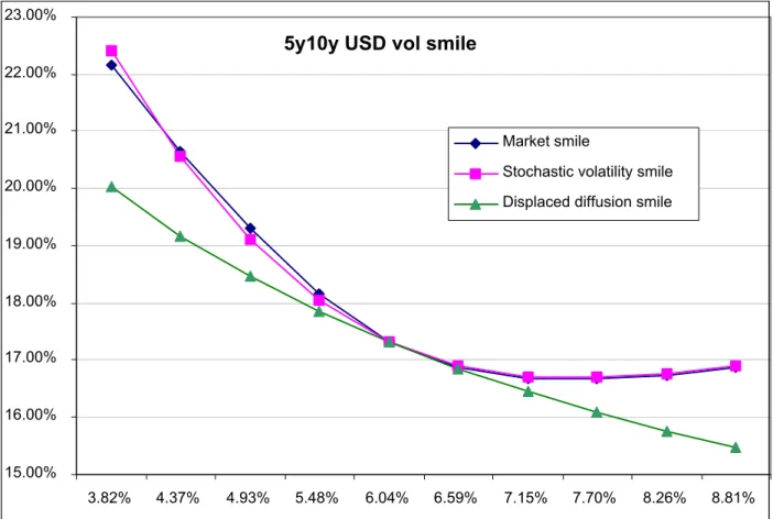
The state of the volatility smile modeling for interest rates is not nearly as advanced as that of the volatility structure modeling. In all fairness, it is technically a much more complicated problem to tackle. Because of that, the impact of various choices of smile dynamics on prices of callable Libor exotics (even as simple as Bermuda swaptions) is poorly understood. State of the art in smile modeling currently involves including stochastic volatility or jumps (or both) in the process for forward Libor rates, typically chosen to be the same for all Libor rates, homogeneous through time and with very simple volatility rate dependence. We present a stochastic volatility forward Libor model later. An example of a volatility smile that this model produces, versus the market smile and versus a simple displaced-diffusion type smile, is given in Figure 2.
5. Forward Libor models
Throughout the paper, Actual/Actual day counting convention is assumed for simplicity, i.e. all day counting fractions are equal to the period length as a fraction of a calendar year. A zero coupon bond paying one dollar at time T,as observed at timet, t≤T,is denoted by P (t, T). A forward Libor rate for the period [T, M], as observed at timet, is defined by
F (t, T, M), P(t, T)−P (t, M) (M −T)P (t, M) .
Let
0 = t0 < t1 <· · ·< tM, τn = tn+1−tn,
be a tenor structure, i.e. a collection of approximately equally spaced (three or six months is common) maturities.
Note that the model’s tenor structure{ti}Mi=0 is potentially different from contract-specific tenor structure {Ti}Ni=1.
We define the n-th forward Libor rate Fn(t) (the n-th “primary” Libor rate) by the expression
Fn(t),F (t, tn, tn+1) = P (t, tn)−P (t, tn+1)
τnP (t, tn+1). , 0≤n < M.
The log-normal model is specified by the following dynamics of each of the forward Libor rates,
dFn(t)/Fn(t) =λn(t)dWTn+1(t), n= 1, . . . , M
−1, t ∈[0, tn], (5.1)
Hereλn(·)is a deterministic function of timeR+→Rn,anddWTn+1(·)is a one-dimensional Brownian motion under theTn+1-forward measure. (We consider a one-dimensional case for brevity.)
The skew-extended forward Libor model introduces a local volatility function φ(x), in-dependent of time, that is applied to each of the Libor rates. The dynamics (under the appropriate forward measures) is given for each Fn by
dFn(t) =λn(t)φ(Fn(t))dWTn+1(t), n= 1, . . . , M
−1, t∈[0, tn]. (5.2)
A popular choice for φ(x) is a linear function
φ(x) =ax+b,
resulting in a “displaced diffusion” type model.
To obtain a stochastic volatility model, we first introduce a process for the stochastic variance
dz(t) = θ(z0−z(t)) dt+εpz(t)dZ(t), z(0) = z0.
Here θ is the mean reversion of variance, ε is the volatility of variance. We assume that Z(·) is independent of the Brownian motions that drive the rates. We add the stochastic volatility on top of the skew-expended forward Libor model to obtain
dFn(t) =pz(t)λn(t)φ(Fn(t))dWTn+1(t), n= 1, . . . , M
−1, t∈[0, tn]. (5.3)
For convenience we define
A special numeraire is usually chosen. We define a discrete money-market numeraire Bt by
Bt0 = 1,
Btn+1 = Btn ×(1 +τnFn(tn)), 1≤n < M,
Bt = P(t, tn+1)Btn+1, t∈[tn, tn+1].
The dynamics of all forward Libor rates under the same measure, the measure associated with Bt,are given by (for the stochastic volatility case)
dFn(t) = z(t)λn(t)φ(Fn(t))
n
X
j=1
1{t<Tj}
τjφ(Fj(t))
1 +τjFj(t)λj(t) dt+
p
z(t)λn(t)φ(Fn(t))dW(t), (5.4)
n= 1, . . . , M −1,
where dW is a Brownian motion under this measure.
The measure P is assumed to be the probability measure associated with the numeraire Bt. The filtration {Ft}∞t=0 is assumed to be generated by the Brownian motion Wt (and properly augmented with the zero-probability events of P).
For the models (5.1) and (5.2), the vector-valued process
¯
F (t) = (F0(t), F1(t), . . . , FM−1(t))
is Markov. For the stochastic volatility model (5.3), the stochastic variance process z(t)
needs to be added to have a Markov process.
The model defined by (5.4) is of the HJM type. In particular, in this model zero coupon discount bonds satisfy the following SDE under the risk-neutral measure,
dP (t, T) =r(t)P(t, T) dt+Σ(t, T)P (t, T) dW(t),
for some bond volatility process{Σ(·, T),0≤T < ∞}.It is also known that we can choose the bond volatility process in such a way that
Σ(t, tn)≡0 for t∈[tn−1, tn]
for any n, 1≤n≤M. We adopt this specification. In particular it implies
P (t, tn) =P (tn−1, t, tn) for t ∈[tn−1, tn], (5.5)
for any n, 1≤n≤M.
6. Valuing callable Libor exotics in a forward Libor model
6.1. Recursion for callable Libor exotics. If a callable contract H0 has not been ex-ercised up to and including time Tn, (“still alive at time Tn”) then it is worth the hold value Hn(Tn). If the callable contract is exercised at time Tn its value is equal to En(Tn). Assuming optimal exercise, the value of the callable Libor exotic H0 at time Tn is then the maximum of the two,
max{Hn(Tn), En(Tn)}.
The value of this payoff at time Tn−1 is then
BTn−1ETn−1B
−1
Clearly this is the value of the Bermuda swaption that can only be exercised at times Tn and beyond, i.e. of the Bermuda swaption Hn−1.These considerations define a recursion
Hn−1(Tn−1) =BTn−1ETn−1B−
1
Tn max{Hn(Tn), En(Tn)}, n=N −1, . . . ,1,
(6.1)
HN−1 ≡0.
The recursion starts at the final time n = N −1 and progresses backward in time. For n= 1 we obtain the value H0(0), the value of the callable that we are after.
This is of course nothing more than a well-known algorithm for pricing American-style options in a backward induction.
Let us denote the exercise region at time Tn by Rn, Rn⊂Ω,
Rn,{ω∈Ω:Hn(Tn,ω)≤En(Tn,ω)}, 1≤n≤N −1. (6.2)
Letη=η(ω)be the index of thefirst time that the exercise region is hit (orN if it is never hit),
η(ω) = min{n≥1 :ω ∈Rn}∧N.
The callable contract value can be re-written as
H0(0) = E0
³
B−Tη1Eη(Tη) ´
= E0
ÃN−1 X
n=η
BT−n+11 Xn
!
.
6.2. Monte-Carlo for American-style options. The problem of pricing American-style options in Monte-Carlo has been considered in [LS98] and [And99]. In the latter, an algorithm for pricing Bermuda swaptions in a forward Libor model was explicitly presented. Extending both algorithms to price callable Libor exotics is a trivial exercise (in theory, not in practice). In this paper we adopt a framework of [LS98].
For more in-depth description of the algorithm for Bermuda swaptions, one can consult [Ped99] or [BM01].
Suppose an estimate of the exercise regions Rn, n˜ = 1, . . . , N−1, is available. Then the estimate of the optimal exercise time index is defined by
˜
η(ω) = minnn≥1 :ω ∈Rn˜ o∧N.
Then, a lower bound on the value of a callable contract can be computed by the standard Monte-Carlo algorithm via the formula
H0(0) ≥ H0˜ (0), (6.3)
˜
H0(0) = E0
ÃN−1 X
n=˜η
BT−n+11 Xn
!
.
The closer the estimated exercise regions Rn˜ to the actual ones, the tighter the lower bound on the value will be.
For each n, 1 ≤ n ≤ N −1, we choose a p-dimensional FTn-measurable “explanatory”
random vector
¯
V (Tn) ={Vm(Tn)}pm=1 ={Vm(Tn,ω)} p m=1.
Also, for each n, 1 ≤ n ≤ N −1, we select two parametric families of R-valued functions fn(v;α) andgn(v;β), v ∈ Rp,α,β
∈A ⊂Rq, q
≥ 1. Without loss of generality we assume that
fn(x; 0) ≡ 0, gn(x; 0) ≡ 0.
We choose special values of the parameters α and β, denoted by αnˆ and βˆn, such that the function fn is a good approximation for the hold value at time Tn as a function of the explanatory vectorV¯(Tn),
Hn(Tn,ω)≈fn¡V¯ (Tn,ω),αnˆ ¢,
and the functiongn is a good approximation for the exercise value at time Tn as a function of the explanatory vectorV¯ (Tn),
En(Tn,ω)≈gn³V¯ (Tn,ω),βˆn
´
.
In particular, the Longstaff-Schwartz estimate of the Rn’s will be of the form
˜
Rn =nω∈Ω:fn¡V¯(Tn,ω),αnˆ ¢ ≤gn³V¯(Tn,ω),βˆn´o, 1≤n≤N −1. (6.4)
This is similar to (6.2) except that the real hold and exercise valuesHn andEn are replaced by their proxies fn¡V¯(Tn)¢ andgn¡V¯(Tn)¢.
Let us describe the algorithm for choosing the values of parametersαn,ˆ βˆn,n= 1, . . . , N−
1, used in (6.4). To get the best possible estimate of the exercise region Rn˜ for each n, we need to approximate the hold value Hn(Tn) as close as possible with one of the functions from the family fn¡V¯(Tn,ω),αn¢, and we need to approximate the exercise value En(Tn)
as close as possible with one of the functions from the familygn¡V¯(Tn,ω),βn
¢
. We use this as an optimality condition to findαn,ˆ βˆn. We optimize the choice ofαn andβn over a set of Monte-Carlo paths pre-simulated for that purpose.
Letωk, k = 1, . . . , K,be a collection of Monte-Carlo simulated paths. For any random vari-ableX,we denote itsk-th simulated value byX(ωk).We choose the optimalfit valueβˆnfrom the condition (a non-linear regression of then-th exercise value on©gn¡V¯(Tn,ωk) ;β¢ªKk=1),
ˆ
βn = arg min
β
K
X
k=1
Ã
BTn(ωk)
N
X
i=n
BT−i1(ωk)Xi(ωk)−gn¡V¯(Tn,ωk) ;β¢
!2 (6.5)
for n= 1, . . . , N−1.
The optimalfit variablesαn, nˆ = 1, . . . , N−1for the hold value are obtained in backward induction. We set
(so that fN ≡ 0 which is consistent with the fact that HN−1 ≡ 0 by definition).Then, for eachn, having computedαn+1,ˆ βˆn+1 on the previous step, we obtain αnˆ from
ˆ
αn = arg min
α
K
X
k=1
³
BTn(ωk)B
−1
Tn+1(ωk) max
n
fn+1¡V¯(Tn+1,ωk),αn+1ˆ ¢, gn+1³V¯ (Tn+1,ωk),βˆn+1
´o
(6.6)
−fn¡V¯(Tn,ωk) ;α¢¢2.
In practice the parametric families fn(·,α) andgn(·,β) are most often chosen to depend linearly on parameters α and β. This makes solving for αnˆ and βˆn from (6.5) and (6.6) as simple as running a linear regression. The linearity assumption does not appear to be restrictive in practice, and we adopt it from now on.
The output of the Longstaff-Schwartz pre-simulation step is an estimate of a set of exercise
regions nRn˜ oN−1
n=1 , and an estimate of the optimal exercise time index ˜η. These are used in obtaining the value (a lower bound) of the contract in the Monte-Carlo simulation via (6.3).
6.3. Differences in the algorithm for CLEs vs. Bermuda swaptions. The scheme presented above is somewhat different from the one typically used for Bermuda swaptions. In particular, for a Bermuda swaption (on a vanillafixed-for-floating swap), there is no need to run a regression on exercise values. The exercise values, being values of plain-vanilla swaps, are available at each exercise date for each path by discounting swap cashflows off
an interest rate curve for the date and path (“off the curve” as we call it). For a general callable Libor exotic this is not the case. The underlying typically contains options, and valuing them on future dates is either impossible (in models without closed form expressions for European options) or too expensive. A better choice, as proposed in the section above, is to use regression to estimate the exercise values.
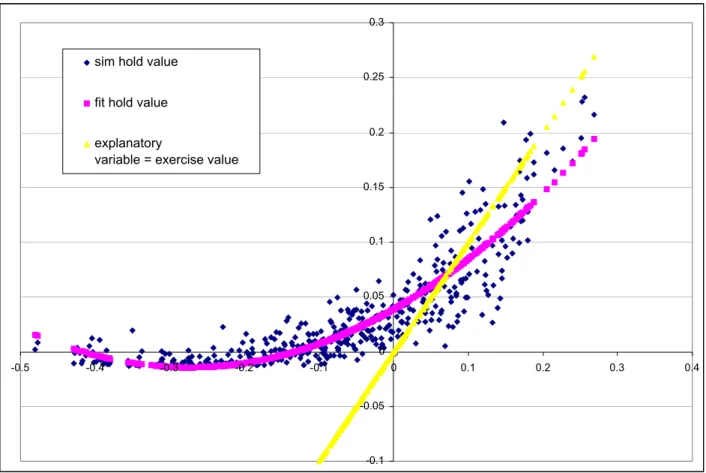
Another simplification that Bermuda swaptions enjoy over more complex callable Libor exotics is the relative ease with which good explanatory variables can be chosen. It is quite clear that for a Bermuda swaption, in regressing the hold value, the value of the underlying swap on each of the exercise dates is very important. It represents an overall level of rates on the exercise date. We show typical results of regressing hold values on exercise values for a Bermuda swaption in Figure 3. Going a bit further it becomes clear that a second important variable is the slope of the interest rate curve on the exercise date (a hold value is an option on rates with different tenors, and therefore their relative values, as measured by the slope, are likely to be important). For callable Libor exotics, the choice of explanatory variables is less clear-cut. We discuss it in the next section.
For the LS algorithm to work, numerical properties of the regression procedure are im-portant. The success of the LS algorithm will depend on how robust and well-behaved the numerical problem of fitting f andg to simulated values is. Overfitting is the main danger. In particular, one should not use an overly rich set of parametric functions in the fitting. The more functions there are to choose from for the optimization procedure, the less robust it generally is. A less robustfitting procedure mayfind afit that is acceptable for the values itfits but behaves completely unreasonably outside the range of fitted values. For example, high-order polynomials will generally be a bad choice as they would react very strongly to the presence of outliers in the simulation.
The danger of overfitting is somewhat increased by the fact that both explanatory variables and parametric families perform basically the same function. To avoid this problem we must separate the roles that parametric families and explanatory variables play. To that effect, we impose the following distinction on the two. We argue for using very simple parametric families (for example, polynomials of degree 2 in multiple variables work well). With simple parametric families, the dangers of overfitting are minimized.
Another reason for using low-order polynomials is given in [GY03]. The result of the paper states that the number of paths required for convergence grows exponentially with the order of polynomials used.
Choosing simple parametric families is not as restrictive as it looks. The parametric families f andg are only used to set exercise regions, see (6.4). The only place where good fit is really required is around the exercise boundary. And that can typically be achieved with simple parametric families.
Since parametric families are simple, one only needs to focus on choosing good explanatory variables. By “good” we mean financially meaningful variables that really drive the future simulated exercise and hold values.
There are no hard and fast rules for choosing explanatory variables. The analogy with Bermuda swaptions should be a good guide. Also, the following considerations should be employed.
• Use financially meaningful explanatory variables;
• Decide what are the primary financial variables affecting exercise values (often the overall level of rates on the exercise date);
• Decide what are the primaryfinancial variables affecting hold values relative to exercise values (often the slope of the rate curve on the exercise date);
• Decide what are the secondary effects and whether they should be accounted for. One requirement on explanatory variables mentioned in Section 6 should be explained in a bit more detail. For the LS algorithm to work, these variables, observed on any exercise time Ti, should be FTi-measurable. What it means is that they should not be “future-looking”.
They should be computable by using only the state of the model i.e. the interest rate curve, as observed up to and at time Ti. This requirement, while seemingly technical, is very important to the success of the algorithm. It comes down to the fact that we one is not allowed to “see into the future” to make our exercise decisions.
between the swap rate and some short-tenor Libor rate. One does not need to include the difference of the rates as an explanatory variable. The short-tenor Libor rate will work just as well. The properly weighted difference of the two will implictly be used in the fitting of parametric families.
The number of explanatory variables one typically needs is pretty small (if they are prop-erly chosen). Two variables per exercise date are usually enough. It is hard to get a noticeable improvement in the lower bound by adding a third variable. It also appears that, almost universally, the two most useful explanatory variables are variables representing an overall level of rates and a slope of the interest rate curve. An overall level of rates is usually well captured by a core swap rate (a rate that fixes on the exercise date and matures when the whole deal matures), or something related to it. The slope is well captured by a short-tenor Libor rate (a 6 month or 1 year tenor) thatfixes on the exercise date, or something related to it.
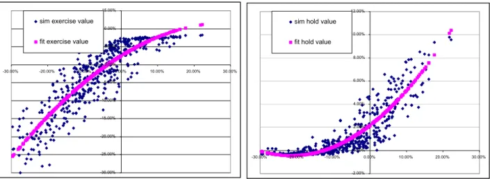
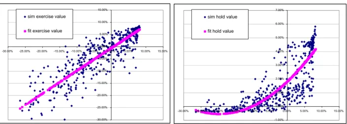
Using a core swap rate, and a short-tenor Libor rate for each exercise date as explanatory variables usually leads to acceptable results. In many cases, however, they can be improved substantially. For a typical CLE, the underlying has interest rate options in it (think of a callable capped floater as an example where the underlying is a collection of caplets) and as such has certain amount of curvature with respect to the level of rates. See the left pane of Figure 4, where simulated exercise values are plotted versus the level of rates. It turns out that using explanatory variables with approximately the same amount of curvature often gives better results. See results in the left pane of Figure 5. One can ask why is that the case, since the parametric functions have curvature, and would be able to match the underlying’s features in the regression even if the explanatory variables were just rates. What comes in play here, however, is the fact that, having chosen simple functions for the parametric families for the purposes of robustness, the “resolution” we get from them is typically insufficient to match the finer features of the dependence of the underlying on the rates. For example, for a callable capped floater, the value of the underlying is capped from above. If we just fit a second-order polynomial to values of such underlying versus the swap rate (see the fitted exercise values on the left pane of Figure 4), thefitted values will not respect the cap, and will happily extend above it. It is especially troublesome given that the poorest fit is achieved where it is needed the most, i.e. around the exercise boundary. This can lead to a sub-par performance of the LS algorithm.
Good fitting of hold values, on the other hand, typically does not require any specially “curved” explanatory variables. The hold values’ curvature is usually well captured by the curvature in parametric functions, especially around the area of interest (around the exercise boundary). These results are plotted in the right panes of Figures 4 and 5.
exactly apply. If the underlying is a strip of options, one does not need to value all options in the underlying, just one (say the one in the middle of the strip). If the speed of valuation is still an issue, one can use formulas that exhibit Black-Scholes like behavior but are faster to compute. For example, the following formula can be used as an approximation:
b(x, K,σ,τ) = −G1¡x−K;σ√τ¢+ (x−K)G0¡x−K;σ√τ¢,
G0(y;v) =
(
1 2e
√
2
v y, y <0, 1− 12e−
√
2
v y, y ≥0,
G1(y;v) =
e √
2 v y
2√2
¡√
2y−v¢ y <0,
e− √
2 v y
2√2
¡
−√2y−v¢ y≥0.
This is the European call option price with strike K, spot x, absolute volatility σ and time to expiry τ in a “model” where the spot process has the probability density
p(y;x, v) = 1
v√2exp
à −
√ 2
v |y−x|
!
, −∞< y <∞.
Volatilities to be used are the forward volatilities of the appropriate Libor rates.
To give an example, consider a callable cappedfloater. The coupon at time Ti is given by (we denoteLi(t) =F (t, Ti, Ti+1))
Ci = min(Li(Ti) +s, c).
The coupon is received against a Libor rate payment,
Xi =δi×(Ci−Li(Ti)).
We note that
Xi = δi×(min(Li(Ti) +s, c)−Li(Ti)) = δi×s−δi×max(Li(Ti)−(c−s))
so the payment is a combination of a fixed rate payment with rate s and a call option on the Libor rate with strike c−s.
For the first explanatory variable we will use an approximate value of the exercise value on each exercise date
V1(Tn) =
NX−1
i=n
δi×P (Tn, Ti+1)×(s−b(Li(Tn), c−s,σni, Ti−Tn)).
Here we use the approximate option formula b(·) (we could have used the Black-Scholes formula if valuation speed was not a concern). The volatility σni is the absolute volatility of the Libor rateLi(·)over the interval [Tn, Ti]as given by the model (or an approximation thereof). To reiterate, very crude approximations can be used here. In the lognormal case we may use
where ¯λ is some average of λn(t) over n and t in (5.1). (We need to multiply it by Li(0)
because the formula asks for the absolute volatility, not a relative one.) For the skew-extended model we may use
σni =φ(Li(0))×λ,¯
and for the stochastic volatility model we may use
σni=pz(Tn)×φ(Li(0))ׯλ. (6.7)
What should we use for our second explanatory variable? In the case of a Bermuda swaption we opted to use a front Libor ratefixing on an exercise date. We can use the same here. Alternatively, we can just use the value of the first coupon payment:
V2(Tn) =δn×P (Tn, Tn+1)×(s−b(Ln(Tn), c−s,σnn,0))
or the last one:
V2(Tn) = δn×P (Tn, TN)×(s−b(LN−1(Tn), c−s,σn,N−1, TN−1−Tn)).
In conjunction with the first explanatory variable, either one will capture the effect of the changing interest rate curve slope well.
For the parametric functions f and g, the second-degree polynomials in V1 and V2 are used.
The approach presented in the example is quite general and can be applied to the vast majority of callable Libor exotics.
Onefinal note is in order. Note that in the stochastic volatility case, we proposed using an explanatory variable that is dependent on the stochastic volatility process. It turns out that this is quite important to do, even for CLEs that do not have optionality in the underlying, like a Bermuda swaption. The stochastic volatility process z(·) can either be incorporated into an explanatory variable like we did it in (6.7), or used as a separate explanatory variable.
6.5. An upper bound in Monte-Carlo simulation. The LS algorithm (as well as other algorithms based on estimating exercise boundaries or exercise decisions) only produces a lower bound on the value of a callable Libor exotic. This is somewhat unsatisfactory, as there is no way of knowing how far offthe lower bound really is from the “true” model value. The problem is especially troubling for more complicated callable Libor exotics where the choice of explanatory variables in not transparent. One can experiment with different choices and try to get the value as high a possible. One is never sure, however, whether the inability to improve a value is due to the fact that it is already close to the true one, or because one was unable to find good explanatory variables.
a good set, the LS algorithm can be run from then on for valuation and risk management purposes.
7. Risk sensitivities of callable Libor exotics: a short overview
Valuation of callable Libor exotics was discussed in the previous sections. With this section we start our discussion of different methods for obtaining various risk sensitivities for callable Libor exotics. The risk sensitivities, also known as Greeks, that we focus on are deltas, vegas and gammas. As a group, they can be thought of as derivatives of the value of a CLE with respect to various market parameters (rates and volatilities).
Conceptually, risk sensitivities should be easy to obtain — just bump the appropriate input and revalue the security. Reality, however, is rather different. Computing Greeks in a Monte-Carlo simulation is a notoriously difficult task. It is a well-known numerical phenomena that the noise, inherently present in Monte-Carlo valuation, affects numerical derivatives (Greeks) significantly more than the underlying value. Interestingly, it is even worse for callable Libor exotics than for other interest rate derivatives. This is a consequence of the way CLEs are valued; we will discuss why this is so in more detail later.
In addition to accuracy, the speed of valuation becomes critical once computation of Greeks enters the picture. The number of various rates/volatilities that a typical CLE is exposed to is large. Computing all these sensitivities takes a lot of time and system resources. Timeliness of computations is, understandably, a big concern for traders.
Most of the rest of the paper is about solving the noise problem. As we can always trade speed of execution for accuracy, savings in valuation time are directly translatable into the quality of risk sensitivity estimates (and vice versa).
Before proceeding any further, let us recall the definitions of Greeks. Deltas are defined as sensitivities of the value of a CLE to small changes in interest rates. Since different parts of the interest rate curve can move relatively independently, interest rate deltas are usually
bucketed. This means that the sensitivity of the value to changed in different parts of the interest rate curve are measured separately. With a forward Libor model, bucketed deltas can naturally be defined as sensitivities to primary Libor ratesFi(0)as defined in Section 5. Vegas are generally defined as sensitivities to small changes in volatilities. What we are most interested in are sensitivities to changes in market volatilities, i.e. term volatilities of caplets and swaptions. Typically, one requires sensitivities to all volatilities that the model was calibrated to. If the model is calibrated to the whole available set of swaptions, vegas are represented by a vega grid, indexed by the swaption’s time to expiration and the maturity of the underlying swap. Note that these vegas are quite different from the sensitivities to model’s own volatilities (λn(·) for the three models defined in Section 5).
Gammas are second order derivatives. They are defined as sensitivities of deltas with respect to interest rate changes. Just like the deltas, they are typically bucketed.
good scenario risk than good local risk, for obvious reasons. Since the focus of this paper is on technical challenges of CLE modeling, we do not pursue the topic of scenario risk further.
8. Exercise boundary and risk sensitivities
To compute risk sensitivities, a market input is shocked by a small amount and the instru-ment is revalued. The base value of the instruinstru-ment is subtracted to get the sensitivity. For callable Libor exotics, revaluing an instrument is a two-stage procedure. First, the exercise boundary is estimated using pre-simulated paths and the LS algorithm. Then, the CLE is valued as a type of a barrier option that pays the exercise value the first time the exercise boundary is crossed (or, rather, the first time an exercise region is hit). The purpose of this section is simple. We will explain why, when computing local risk sensitivities, we do not need to perform thefirst step, the exercise boundary estimation. We can just reuse the exercise boundary that was obtained during the base valuation of the CLE.
Here we only explain the intuition behind this result. A formal proof is given in [Pit03]. The advantages of not having to recompute the exercise boundary for each Greek calcu-lation are clear. First, it is faster. Typically, estimation of the exercise boundary takes as much time as valuation in post-simulation. Since the boundary only needs to be estimated once, roughly 50% of valuation time for each Greek computation is saved.
The other advantage is noise reduction. As a new boundary is not estimated with every input bumped, the noise from errors involved in estimating the boundary never enters the final result.
The basic reason why we do not have to estimate the exercise boundary is this. The exercise boundary obtained for the base valuation is optimal. Optimality implies that the boundary’s first order sensitivity to any input that affects it is zero (first order optimality condition). So, when some input is bumped, its effect on the exercise boundary is only second-order. This means that in the limit, we can keep the same exercise boundary.
Another way of looking at this is to realize that this is a consequence of a smooth pasting condition for the optimal exercise boundary in valuation of American style options.
Here is a “proof” of our statement. Suppose we would like to compute sensitivity to parameter x, whose current value is x0. For each x, there is an optimal exercise boundary ζ(x).We denote the value of a CLE for a given value of the parameterxand some arbitrary boundary ζ by h(ζ, x). Then, the actual CLE value, if the parameter in question is x, is equal to h(ζ(x), x).The sensitivity to x is then equal to
∂
∂xh(ζ(x), x)
¯ ¯ ¯ ¯ x=x0 = ∂
∂ζh(ζ, x0)
¯ ¯ ¯ ¯
ζ=ζ(x0)
× ∂x∂ ζ(x)
¯ ¯ ¯ ¯ x=x0 + ∂
∂xh(ζ(x0), x)
¯ ¯ ¯ ¯ x=x0 .
Note that, sinceζ(x0) is the optimal boundary for the CLE, we have ∂
∂ζh(ζ, x0)
¯ ¯ ¯ ¯
ζ=ζ(x0) = 0.
Hence, the full derivative of h with respect to x is equal to the partial one while keeping the exercise boundary constant.
9. Why CLE Greeks are hard to compute
to, say, European swaptions’ (also computed in a Monte-Carlo simulation of course). It is important to understand the reason for this. Apart from satisfying intellectual curiosity, such knowledge should help us design algorithms that produce cleaner deltas.
Armed with the estimated exercise regions and the optimal exercise index ˜η(·), the value of a callable Libor exotic is given by
˜
H0 =J−1 J
X
j=1 N−1
X
i=1
h
BT−i+11 (ωj)Xi(ωj) 1i≥˜η(ωj)
i
,
where simulated paths (for the post-simulation) are denoted byωj, j = 1, . . . , J.The depen-dence of the simulated CLE value H0˜ on small changes in (for example) time-zero primary Libor rates Fm(0), m = 0, . . . , M −1, comes from a number of different sources (we will discuss this issue in the context of deltas, but the same considerations apply to vegas as well). First, there is the dependence of BT−i+11 (ωj) on Libor rates. This dependence is very smooth, as clear from the formula for the numeraire. Then there is the dependence of payments Xi(ωj). For many important classes of CLEs this is also smooth (analytic for Bermuda swaptions; continuous for callable inverse floaters and the like). Finally there is the dependence of “exercise indicators” 1i≥η˜(ωj) on the rates. It should be clear that these
indicators do not depend smoothly on the changes in rates at all. And these are actually the culprit of our problems with deltas. Non-smooth dependence like this produces noisy deltas. We note that these indicators are not present in valuation formulas for, say, Eu-ropean swaptions. The indicators specify which coupons have to be added to the exercise value for each simulated path. Being binary “yes/no” indicators they cannot vary smoothly with rates. A small change in rates can add/subtract a whole payment for a particular path. Figure 6 demonstrates the problem visually. If a path of interest rates passes sufficiently close to the exercise boundary, then a small change in the initial values of primary Libor rates {Fm(0)} can push the path outside of the exercise region for one of the exercise dates. A whole payment is lost as a result.
In effect, in a Monte-Carlo simulation, a callable Libor exotic behaves like a barrier option in a Monte-Carlo simulation. This behavior is not a result of having only a suboptimal
exercise boundary coming from the LS algorithm. In fact, had we used the absolute optimal exercise boundary, we would still have the same problem — for some paths, a whole payment will be added/lost under a bump. Differentiating discontinuous functions is hard!
10. Computing deltas in the same simulation
As explained in the previous section, the standard “bump and revalue” method of ob-taining deltas can run into problems. The valuation algorithm treats callable Libor exotics as barrier options. This introduces a lot of noise in sensitivities calculations. However, if one steps back and looks at a callable Libor exotic, it actually does not look like a barrier option at all. Because of the optimality of exercise condition, hold and exercise values are continuous across the exercise boundary. So the problem discussed in the previous section does not appear to be intrinsic to the instrument, but only to the method used to compute deltas.
interest rates, it was first proposed in [GZ99]. The method was extended to callable Libor exotics in [Pit03].
The method allows one to compute deltas of a CLE in the same simulation as the value. This speeds up the valuation of Greeks considerably. More importantly, the resulting deltas are significantly less noisy. The latter is the result of a numerical scheme that avoids rep-resenting CLEs as barrier-type structures. As reported in [Pit03], the standard errors for pathwise deltas can be as much as 5-6 times less than for the “bump and revalue” ones, resulting computation time savings by a factor of 25 to 35.
Before carrying on, we note that the method does not work for CLEs whose coupons are discontinuous functions of rates (such as callable range accruals). For such CLEs, a less advantageous (but still better than “bump and revalue”) approach of likelihood ratio deltas can be applied. For details see [GZ99] and [Pit03].
Let us define pathwise deltas and outline the main steps in applying the pathwise deltas method to CLEs (for details and proofs see [Pit03]). The main formula for the method is (10.6) below, with pathwise deltas of forward Libor rates defined by (10.2) or (10.3).
10.1. Pathwise deltas. For any random payoff X, them-th delta is defined by
∆mX , ∂X
∂Fm(0),
where {Fm(t)} is the set of primary Libor rates.
Suppose X = V ¡F¯(T)¢ for a (reasonably smooth) deterministic function V (x), x = (x0, . . . , xM−1). Then
∆mV ¡F¯(T)¢ =
MX−1
i=0
∂V ¡F¯(T)¢
∂xi ·∆mFi(T). (10.1)
The value of the payoff X at time 0is equal to
E0¡BT−1X¢,
and its delta
∆mE0
¡
BT−1X¢ = E0
¡ ∆m
¡
BT−1V ¡F¯(T)¢¢¢ = E0
¡ ∆m
¡
BT−1¢V ¡F¯(T)¢¢ +E0¡BT−1∆mV ¡F¯(T)¢¢.