The shock-acoustic waves generated by earthquakes

Annales

Geophysicae

The shock-acoustic waves generated by earthquakes

E. L. Afraimovich, N. P. Perevalova, A. V. Plotnikov, and A. M. Uralov

Institute of Solar-Terrestrial Physics SD RAS, P. O. Box 4026, Irkutsk, 664033, Russia Received: 6 July 2000 – Revised: 5 February 2001 – Accepted: 6 March 2001

Abstract. We investigate the form and dynamics of shock-acoustic waves generated by earthquakes. We use the method for detecting and locating the sources of ionospheric impul-sive disturbances, based on using data from a global network of receivers of the GPS navigation system, and require no a priori information about the place and time of the associ-ated effects. The practical implementation of the method is illustrated by a case study of earthquake effects in Turkey (17 August and 12 November 1999), in Southern Sumatra (4 June 2000), and off the coast of Central America (13 Jan-uary 2001). It was found that in all instances the time period of the ionospheric response is 180–390 s, and the amplitude exceeds, by a factor of two as a minimum, the standard de-viation of background fluctuations in total electron content in this range of periods under quiet and moderate geomag-netic conditions. The elevation of the wave vector varies through a range of 20–44◦_{, and the phase velocity (1100–}

1300 m/s) approaches the sound velocity at the heights of the ionospheric F-region maximum. The calculated (by neglect-ing refraction corrections) location of the source roughly cor-responds to the earthquake epicenter. Our data are consistent with the present views that shock-acoustic waves are caused by a piston-like movement of the Earth’s surface in the zone of an earthquake epicenter.

Key words. Ionosphere (ionospheric disturbances; wave propagation) – Radio science (ionospheric propagation)

1 Introduction

A plethora of publications have been devoted to the study of the ionospheric response to disturbances arising from impul-sive forcing on the Earth’s atmosphere. It was found that in many cases a high proportion of the energy of the initial at-mospheric disturbance is concentrated in the acoustic shock wave. Large earthquakes also provide a natural source of im-pulsive forcing.

Correspondence to: E. L. Afraimovich (afra@iszf.irk.ru)

These investigations also have important practical impli-cations since they furnish a means of substantiating reliable signal indications of technogenic effects,which is necessary for the construction of an effective global radiophysical sys-tem for the detection and localization of these effects. Es-sentially, existing global systems with such a purpose use different processing techniques for infrasound and seismic signals. However, in connection with the expansion of the geography and the types of technogenic impact on the envi-ronment, very challenging problems, heretofore, have been those which improve the sensitivity of detection and the re-liability of measured parameters of the sources of impacts, based also on using independent measurements of the entire spectrum of signals generated during such effects.

To solve the above problems requires reliable information about fundamental parameters of the ionospheric response to the shock wave, such as the amplitude and the form, the pe-riod, the phase and group velocity of the wavetrain, as well as angular characteristics of the wave vector. Note that for naming the ionospheric response of the shock wave, the lit-erature uses terminology incorporating a different physical interpretation, among them the term ‘shock-acoustic wave’ (SAW) (Nagorsky, 1998). For convenience in this paper, we shall use this term despite the fact that it does not reflect es-sentially the physical nature of the phenomenon.

There is a wide scatter of published data on the main pa-rameters of SAWs generated during industrial explosions and earthquakes. The oscillation period of the ionospheric re-sponse of SAWs varied from 30 to 300 s, and the propa-gation velocity fluctuated from 700 to 1200 m/s (Nagorsky, 1998; Fitzgerald, 1997; Calais et al., 1998; Afraimovich et al., 1984; Blanc and Jacobson, 1989).

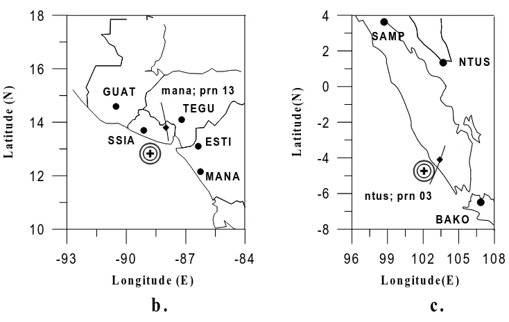
Table 1. General information about earthquakes

N Epicenter Data

t0

(UT)

Depth (km)

Magnitude mb Ms Mw

DST (nT) 1 40.70 N, 29.99 E 17 Aug 1999 (DAY 229) 00:01:39 17 6.3 7.8 7.4 −14 2 40.79 N, 31.11 E 12 Nov 1999 (DAY 316) 16:57:20 10 6.5 7.5 7.1 −44 3 4.72 S, 102.1 E 4 Jun 2000 (DAY 156) 16:28:26 33 6.8 8.0 7.7 +8 4 12.83 N, 88.79 W 13 Jan 2001 (DAY 013) 17:33:29 39 – – 7.6 +4

this method is sufficient to detect the SAW reliably; how-ever, difficulties emerge for localizing the region where the detected signal is generated. These problems are caused by the multiple-hop character of HF signal propagation. This provides no chance of deriving reliable information about the phase and group velocities of the SAW propagation, of estimating angular characteristics of the wave vector, and, further still, of localizing the SAW source.

Using the method of transionospheric sounding with VHF radio signals from geostationary satellites, a number of ex-perimental data on SAW parameters were obtained in mea-surements of the Faraday rotation of the plane of signal po-larization, which is proportional to a total electron content (TEC) along the line connecting the satellite-borne transmit-ter with the receiver (Li et al., 1994).

A common drawback of the above-mentioned methods when determining the SAW phase velocity is the necessity of knowing the time of events, since this velocity is inferred from the SAW delay with respect to the time of events, as-suming that the velocity is constant along the propagation path, which is quite contrary to fact. For determining the above-mentioned fairly complete set of SAW parameters, it is necessary to have appropriate spatial and temporal resolu-tion, which cannot be ensured by the existing very sparse networks of ionosondes, oblique-incidence radio sounding paths, and incoherent scatter radars.

The advent of the Global Positioning System (GPS), plus the subsequent creation of extensive networks of GPS sta-tions (at least 757 sites as of November 2000), with their data being now available via the Internet, has opened up a new era in remote ionospheric sensing.

Currently, some authors have embarked on an intense de-velopment of methods for detecting the ionospheric response of strong earthquakes (Calais and Minster, 1995), rocket launchings (Calais and Minster, 1996), and industrial surface explosions (Fitzgerald, 1997; Calais et al., 1998). In the cited references, the SAW phase velocity was determined by the ‘crossing’ method, by estimating the time delay of SAW ar-rival at subionospheric points corresponding to different GPS satellites observed at a given time. However, the accuracy of such a method is rather low because the altitude at which the subionospheric points are specified is determined in a crude way.

The goal of this paper is to describe a method for de-termining parameters of the SAW generated by earthquakes (including the phase velocity, angular characteristics of the

SAW wave vector, the direction towards the source, and the source location) using GPS-arrays whose elements can be chosen out of a large set of GPS stations from the global GPS network. Section 2 presents a description of the exper-imental geometry, and general information about the earth-quakes under consideration. The proposed method is briefly outlined in Sect. 3. Results of measurements of SAW pa-rameters from different GPS arrays during earthquakes are presented in Sect. 4. Section 5 is devoted to the discussion of experimental results, including analytical simulation results.

2 The geometry and general characterization of experi-ments

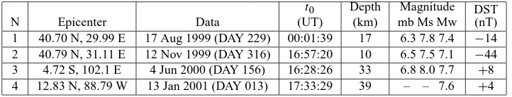
Detection results on two earthquakes in Turkey (17 August and 12 November 1999), in Southern Sumatra (4 June 2000), and off the coast of Central America (13 January 2001) are presented below. The information about the earthquakes was acquired via the Internet (http://earthquake.usgs.gov). Gen-eral information about these earthquakes is presented in Ta-ble 1 (including the time of the main shock,t0, in the uni-versal time UT, the position of the earthquake epicenter, the depth and the magnitude, as well as the level of geomagnetic disturbance from the data onDst-variations). It was found that the deviation ofDstfor the selected days was quite mod-erate, which enabled the SAWs to be identified.

Figure 1 illustrates the experimental geometry during the earthquakes in Turkey (a), off the coast of Central America (b), and in Southern Sumatra (c).

In spite of the small number of GPS stations in the earth-quake area, we were able to use a sufficient number of them for the implementation of the proposed method. Table 2 presents the geographic coordinates of the GPS stations used as GPS array elements.

3 Methods of determining shock-acoustic wave charac-teristics using GPS-arrays

T U R K E Y E A R T H Q U A K E S

A N K R

N IC O

B S H M

G IL B T E L A

R A M O K A B R

K A T Z

2 4 2 7 3 0 3 3 3 6 3 9

L o n g itu d e (E ) 3 0

3 2 3 4 3 6 3 8 4 0 4 2

L

a

ti

tu

d

e

(N

)

K 1 K 2 D A Y 3 1 6

g ilb ; p rn 3 0

a .

b sh m ; p rn 0 6

E A R T H Q U A K E O F F C O A S T O F C E N T R A L A M E R IC A A N D S O U T H E R N S U M A T R A

-9 3 -9 0 -8 7 -8 4

L o n g itu d e (E ) 1 0

1 2 1 4 1 6 1 8

L

a

ti

tu

d

e

(

N

) _{G U A T}

T E G U

S S IA

M A N A E S T I m an a ; prn 13

9 6 9 9 1 0 2 1 0 5 1 0 8

L o n g itu d e (E ) -8

-6 -4 -2 0 2 4

L

a

ti

tu

d

e

(N

)

n tu s ; prn 03

N T U S S A M P

B A K O

b . c .

D A Y 2 2 9

Fig. 1. Experimental geometry during the earthquakes in Turkey – (a). Crosses show the positions of the earthquake epicenters. Solid

curves represent the trajectories of the subionospheric points for each GPS satellite at the heighthi =400 km. Dark diamonds along the

trajectories correspond to the coordinates of the subionospheric points at timetpof a maximum deviation of the TEC. Heavy dots and large

lettering show the location and the names of the GPS stations, while lower-case letters along the trajectories refer to station names and PRN numbers of the GPS satellites for these trajectories. Asterisks mark the source location at 0 km altitude inferred from the data from the GPS arrays. Numbers at the asterisks correspond to the respective day numbers. Straight dashed lines that connect the expected source and the subionospheric point represent the horizontal projection of the wave vectorKt. The scaling of the coordinate axes is chosen from

Table 2. GPS-sites and location

N Sites

Geograph. latitude

Geograph.

longitude N Sites

Geograph. latitude

Geograph. longitude

1 ANKR 39.887 32.759 9 TEGU 14.090 −87.206

2 BSHM 32.778 35.022 10 SSIA 13.697 −89.117

3 GILB 32.479 35.416 11 MANA 12.149 −86.2489

4 KABR 33.022 35.145 12 GUAT 14.590 −90.520

5 KATZ 32.995 35.688 13 ESTI 13.100 −86.3621

6 NICO 35.141 33.396 14 SAMP 3.622 98.715

7 RAMO 30.597 34.763 15 NTUS 1.346 103.680

8 TELA 32.067 34.780 16 BAKO −6.491 106.849

formula for the total electron content (I)

I = 1 40.308

f₁2f₂2

f₁2−f₂2

[(L1λ1−L2λ2)+const+nL] (1)

whereL1λ1andL2λ2are additional paths of the radio sig-nal caused by the phase delay in the ionosphere, (in m);L1 andL2 represent the number of phase rotations at the fre-quenciesf1 andf2;λ1andλ2stand for the corresponding wavelengths, (in m); const is the unknown initial phase am-biguity, (in m); andnL are errors in determining the phase path, (in m).

Phase measurements in the GPS can be made with a high degree of accuracy corresponding to the error of TEC deter-mination of at least 1014m−2when averaged on a 30-second interval, with some uncertainty of the initial value of TEC, however. This makes possible the detection of ionization ir-regularities and wave processes in the ionosphere over a wide range of amplitudes (up to 10−4of the diurnal TEC varia-tion) and periods (from 24 hours to 5 min). The unit of TEC, TECU, is equal to 1016m−2_{; it is commonly accepted in the} literature, and will be used hereafter.

A convenient way of determining the ionospheric response delay of the shock wave involves the frequency Doppler shift F from TEC series, obtained by formula (1). Such an ap-proach is also useful in comparing TEC response characteris-tics from the GPS data with those obtained by analyzing VHF signals from geostationary satellites, as well as in detecting the shock wave in the HF range. For an approximation suf-ficient for the purpose of our investigation, a corresponding relationship was obtained by Davies (1969)

F =13.5·10−8I_t0/f (2) whereI_t0stands for the time derivative of TEC. Relevant re-sults derived from analyzing theF (t ) variations calculated for the ‘reduced’ frequency of 136 MHz are discussed in Sect. 4.

The correspondence of space-time phase characteristics, obtained through transionospheric soundings, with local char-acteristics of disturbances in the ionosphere, was considered in detail in a wide variety of publications (Afraimovich et al., 1992; Mercier and Jacobson, 1997) and is not analyzed

at length in this study. The most important conclusion of the cited references is the fact that, the extensively exploited model of a ‘plane phase screen’ disturbance1I (x, y, t )of TEC, faithfully copies the horizontal part of the correspond-ing disturbance of local electron concentration1N (x, y, z, t ), independent of the angular position of the source, and thus, can be used in experiments for measuring the TEC distur-bances.

However, the TEC response amplitude experiences a strong azimuthal dependence caused by the integral charac-ter of a transionospheric sounding. As a first approximation, the transionospheric sounding method is responsive only to Traveling Ionospheric Disturbances (TIDs), with the wave vector Kt perpendicular to the directionr, which is along the Line-of-Sight (LOS) from the receiver to the satellite. A corresponding condition for elevationθand azimuthαof an arbitrary wave vectorKt normal to the directionr, has the form

θ=arctan(−cos(αs−α)/tanθs) (3) whereαs is the azimuthal angle measured east to north, and θs is the angle of elevation of the satellite at the receiver.

We used formula (3) to determine the elevationθ ofKt from the known mean value of azimuthαby Afraimovich et al. (1998) – see Sects. 3.2 and 4.

3.1 Detection and determination of the horizontal phase ve-locity and the direction of the SAW phase front along the ground by GPS-arrays

In the simplest form, space-time variations of the TEC 1I (t, x, y)in the ionosphere, at each given timet, can be represented in terms of the phase interference pattern that moves without a change in its shape (the solitary, plane trav-elling wave)

disturbance. The vectorK is a horizontal projection of the full vectorKt.

At this point, it is assumed that in the case of small spatial and temporal increments (the distances between GPS-array sites are less than the typical spatial scale3 of TEC vari-ation, and the time interval between counts is less than the corresponding time scale), the influence of second deriva-tives can be neglected. The following choices of GPS-arrays meet these requirements.

We now summarize briefly the sequence of data process-ing procedures. Out of a large number of GPS stations, three sites (A, B, C) are selected within distances not exceeding about one-half of the expected wavelength3of the pertur-bation. Site B is taken to be the center of a topocentric refer-ence frame whose axisxis directed east, and whose axisyis directed north. The receivers in this frame of reference have the coordinates(xA, yA), (0,0), (xC, yC); such a configu-ration of the GPS receivers represents the GPS-array with a minimum number of the required elements. In regions with a dense network of GPS sites, we can obtain a large variety of GPS-arrays of a different configuration, enabling the ac-quired data to be checked for reliability; in this paper, we have exploited this possibility.

The input data includes series of slant TEC valuesIA(t ), IB(t ),I(t ), as well as the corresponding series of elevation valuesθs(t ), and the azimuthαs(t )of the LOS. For determin-ing SAW characteristics, continuous series of measurements ofIA(t ),IB(t ),IC(t )are selected with a length of at least a one-hour interval, which includes the time of a earthquake.

To eliminate spatio-temporal variations of the regular iono-sphere, as well as trends introduced by the orbital motion of the satellite, a procedure involving a preliminary smoothing of the initial series with the selected time window is used to remove the trend. This procedure is better suited to the de-tection of a single pulse signal (N-wave) than the frequently used band-pass filter (Li et al., 1994; Calais and Minster, 1995, 1996; Fitzgerald, 1997; Calais et al., 1998). A lim-itation of the band-pass filter is the oscillatory character of the response which prevents it from reconstructing the form of theN-wave.

Elevationθs(t )and azimuthαs(t )values of the LOS are used to determine the location of the subionospheric point, as well as to calculate the elevationθ of the wave vectorKt of the disturbance from the known azimuthα(see formula (3)). The most reliable results from the determination of SAW parameters correspond to high values of elevationsθs(t )of the LOS because sphericity effects become reasonably small. In addition, there is no need to convert the slant TEC1I (t ) to a ‘vertical’ value. In this paper, all results were obtained for elevationsθs(t )larger than 30◦.

Since the distance between GPS-array elements (from sev-eral tens of kilometers to a few hundred kilometers) is much smaller than the distance to the GPS satellite (over 20000 km), the array geometry at the height of the ionosphere is identical to that on the ground.

Figure 2a shows typical time dependencies of a slant TEC I (t ) at the GPS-array BSHM station near the area of the

earthquake of 17 August 1999 (heavy curve), one day be-fore and after the earthquake (thin lines). For the same days, panel b shows TEC variations1I (t )after removal of a linear trend and smoothing by averaging over a sliding window of 5 min. Variations in frequency Doppler shiftF (t ), ‘reduced’ to the sounding signal frequency of 136 MHz for three sites of the array (KATZ BSHM GILB) on 17 August 1999, are presented in panel c.

Figure 2 shows that fastN-shaped oscillations, with a typi-cal period of about 390 s, are distinguished among slow TEC variations. The oscillation amplitude (up to 0.12 TECU) is far in excess of the background TEC fluctuation intensity, as seen on the days before and after the earthquake. Variations in frequency Doppler shiftF (t )for spatially separated sites (KATZ BSHM GILB) are well correlated but are shifted rela-tive to each other by an amount well below the period, which permits the SAW propagation velocity to be unambiguously determined. The 30 s sampling rate of the GPS data is not quite sufficient for determining small shifts of such signals with an adequate accuracy for different sites of the array. Therefore, we used a parabolic approximation of theF (t )-oscillations in the neighborhood of minimumF (t ), which is quite acceptable when the signal/noise ratio is high.

Taking into account the good signal/noise ratio (better than 1), and knowing the coordinates of the array sites A, B and C, we determine the horizontal projection of the phase veloc-ityVh from time shifts tp of a maximum deviation of the frequency Doppler shiftF (t ). Preliminarily measured shifts are subjected to a linear transformation with the purpose of calculating shifts for sites spaced relative to the central site northwardN and eastwardE. This is followed by a calcula-tion of theE- andN-components ofVxandVy, as well as the directionαin the range of angles 0–360◦and the modulusVh of the horizontal component of the SAW phase velocity

α=arctan(Vy/Vx) (5)

Vh= |VxVy|(Vx2+Vy2)

−1/2

whereVy,Vx are the velocities with which the phase front crosses the axes x and y. The orientationα of the wave vectorK, which is coincident with the propagation azimuth of the SAW phase front, is calculated unambiguously in the range 0–360◦, subject to the condition that arctan(Vy/Vx)is calculated with regard to the sign of the numerator and de-nominator.

The above method for determining the SAW phase veloc-ity neglects the correction for orbital motion of the satellite because the estimates ofVh, obtained below, exceed an order of magnitude, as a minimum, of the velocity of the subiono-spheric point at the height of the ionosphere for elevations θs >30◦ (Afraimovich et al., 1998).

0 .0 0 .2 0 .4 0 .6 0 .8

0

5

1 0

0 .0

0 .2

0 .4

0 .6

-0 .1 6

0 .0 0

0 .1 6

1 7 .0

1 7 .2

1 7 .4

0

5

1 0

1 7 .0

1 7 .2

1 7 .4

-0 .1 2

0 .0 0

0 .1 2

I(t), 1 0

_m

a.

b .

c.

1 29 1

1 4 1

29

Y AKA

F A I R

0 .0

0 .2

0 .4

0 .6

U T , h o u r

-0 .0 5

0 .0 0

0 .0 5

1 7 .0

1 7 .2

1 7 .4

U T , h o u r

-0 .0 3

0 .0 0

0 .0 3

M A C 1

P R N 2 2 P R N 2 9

F (t), H z F (t), H z

I(t), 1 0

m

B S H M ; P R N 6 G IL B ; P R N 3 0 D A Y 2 29

B S H M G IL B G IL B K A B R

K A T Z T E L A

∆ ∆

D A Y 2 28 D A Y 3 15

P R N 6 P R N 30 D A Y 2 28

D A Y 23 0

1 7.08 .1 99 9 12 .1 1.1 99 9

I(t), 1 0

m

I(t), 1 0

m

D A Y 3 17 D A Y 31 5

d .

e.

f.

D A Y 23 0 D A Y 31 7

B S H M ; P R N 6 G IL B ; P R N 3 0

D A Y 22 9 D A Y 31 6

T U R K E Y E A R T H Q U A K E S

Fig. 2. Time dependencies of slant TECI (t )at one of the three sites of the GPS-array in the area of the earthquakes on 17 August and

From the delay1t =tp−t0and the known path length between the earthquake focus and the subionospheric point, we also calculated the SAW mean velocityVa, in order to compare our estimates of the SAW phase velocity with the usually used method of measuring this quantity.

3.2 Determination of the wave vector elevationθ and the velocity modulusVt of the shock wave

Afraimovich et al. (1992) showed that for the Gaussian ion-ization distribution, the TEC disturbance amplitude (M) is determined by the aspect angle γ between the vectorsK_t andr, as well as by the ratio of the wavelength of the dis-turbance3to the half-thickness of the ionization maximum hd

M∝exp −π 2_h2

dcos 2_γ

32_cos2_θ s

!

. (6)

In the case under consideration (see below), for a phase ve-locity on the order of 1 km/s and for a period of about 200 s, the wavelength3is comparable with the half-thickness of the ionization maximumhd. When the elevationsθsare 30◦, 45◦, 60◦, the ‘beam-width’ M(γ ), at the 0.5 level, is 25◦, 22◦and 15◦, respectively. Ifhdis twice as large as the wave-length, then the beam tapers to 14◦, 10◦and 8◦, respectively. The beam-width is sufficiently small that the aspect condi-tion (3) restricts the number of beam trajectories to the satel-lite, for which it is possible to detect, with reliably, the SAW response in the presence of noise (near the anglesγ =90◦). On the other hand, formula (3) can be used to determine the elevationθof the wave vectorKt of the shock wave at the known value of the azimuthα(Afraimovich et al., 1998). Hence, the phase velocity modulusVt can be defined as

Vt =Vhcos(θ ) (7)

The above values of the widthM(γ )determine the error of calculation of the elevationsθ(of the order of 20◦to the above conditions).

3.3 Determining the position of the SAW source without regard for refraction corrections

The ionospheric region that is responsible for the main con-tribution to TEC variations lies in the neighborhood of the maximum of the ionosphericF-region, which does deter-mine the heighthi of the penetration point. When select-inghi, it should be taken into consideration that the decrease in electron density, with height above the main maximum of the F2-layer, proceeds much slower than below this max-imum. Since the density distribution with height is essen-tially a ‘weight function’ of the TEC response to a wave dis-turbance (Afraimovich et al., 1992), it is appropriate to use, ashi, the value exceeding the true height of the layerhmF2 maximum by about 100 km. hmF2 varies between 250 and 350 km depending on the time of day and on some geophysi-cal factors which, when necessary, can be taken into account

if additional experimental data and current ionospheric mod-els are available. In all calculations that follow,hi =400 km is used.

To a first approximation, it can be assumed that the imag-inary detector, which records the ionospheric SAW response in TEC variations, is located at this altitude. The horizontal extent of the detection region, which can be inferred from the propagation velocity of the subionospheric point as a conse-quence of the orbital motion of the GPS satellite (on the or-der of 70–150 m/s; see Pi at al., 1997), and from the SAW period (on the order of 200 s; see Sect. 4), does not exceed 20–40 km, which is far smaller than its ‘vertical size’ (on the order of the half-thickness of the ionization maximumhd).

From the GPS data, we can determine the coordinatesXs andYs of the subionospheric point in the horizontal plane X0Y of a topocentric frame of reference centered on the point B(0,0) at the time of a maximum TEC deviation, caused by the arrival of the SAW at this point. Since we know the angular coordinatesθandαof the wave vectorKt, it is possible to determine the location of the point at which this vector intersects the horizontal planeX00Y0_{at the height}

hw of the assumed source. Assuming a rectilinear propaga-tion of the SAW from the source to the subionospheric point and neglecting the Earth sphericity, the coordinatesXw and Yw of the source in a topocentric frame of reference can be defined as

Xw =Xp−(hi −hw)

cosθsinα

sinθ (8)

Yw =Yp−(hi−hw)

cosθcosα

sinθ (9)

The coordinatesXwandYw, thus obtained, can readily be recalculated to the values of the latitude and longitude (φw andλw) of the source. For SAW generated during earth-quakes, industrial explosions and underground tests of nu-clear devices,hw is taken to be equal to 0 (the source lying at the ground level).

4 Results of measurements

Hence, using the transformations described in Sect. 3, we obtain the parameters set determined from TEC variations and characterizing the SAW (see Table 3).

Let us consider the results derived from analyzing the iono-spheric effect of SAW during earthquake 17 August 1999, obtained at the array (KATZ, BSHM, GILB) for PRN 6 (at the left of Fig. 2, and line 2 in Table 3).

Table 3. The parameters of shock-acoustic waves

No. Sites tp

(UT)

1t, sec.

T, sec.

AI,

TECU

AF,

Hz

θ,◦ α,◦ Vh,

m/s

Vt,

m/s

Vα,

m/s

ϕw,◦ λw,◦

17 Aug 1999;t0=00:01:39 UT

1 KABR BSHM KATZ 00:21:04 00:21:19 1165 1180 360 300 0.15 0.14 0.037 0.049

24.9 155 1296 1174 873

862 39.6 26.4 2 GILB KATZ BSHM

00:21:54 1215 390 0.12 0.043 26.1 154 1307 1174 868 39.1

25.9

3 KATZ

KABR GILB

00:21:23 1184 360 0.19 0.05 25.1 155 1303 1179 854 39.5

26.4

4 TELA

BSHM GILB

00:22:14 1235 360 0.1 0.026 19.9 161 1238 1164 894 41.5

26.1

5 P

354 0.14 0.04 24.1 156 1286 1173 870 39.9

26.2 12 Nov 1999;t₀=16:57:20 UT

6 KABR BSHM GILB 17:12:58 17:13:21 938 961 180 180 0.06 0.07 0.027 0.021

29.5 194 1285 1119 807

787 42.2 30.1 7 TELA KABR GILB

17:14:09 1009 210 0.097 0.021 43.8 180 1487 1073 838 39.4

28.6

8 GILB

BSHM TELA

17:13:39 979 210 0.09 0.022 39.6 184 1663 1280 817 40.1

29.1

9 P

195 0.079 0.023 37.6 186 1478 1157 812 40.5

29.2 4 Jun 2000;t0=16:28:26 UT

10 SAMP NTUS BAKO 16:46:12 16:42:16 16:49:16 1092 856 1276 270 270 240 0.1 0.5 0.06 0.04 0.09 0.02 558 503 642

13 Jan 2001;t0=17:33:29 UT

11 TEGU ESTI MANA 17:45:11 17:46:30 17:47:21 851 930 981 240 210 270 0.09 0.09 0.2 0.03 0.03 0.05 591 488 440

The amplitude of a maximum frequency Doppler shiftAF, at the ‘reduced’ frequency of 136 MHz, was found to be 0.04 Hz. In view of the fact that the shift F is inversely pro-portional to the sounding frequency squared (Davies, 1969), this corresponds to a Doppler shift at the working frequency of 13.6 MHz and the equivalent oblique-incidence sounding path of aboutAF =4 Hz.

Solid curves in Fig. 1a represent the trajectories of the subionospheric points for each GPS satellite at the height hi =400 km during the time interval 0.0–0.8 UT for 17 Au-gust 1999, and 17.0–17.4 UT for 12 November 1999. Dark diamonds along the trajectories correspond to the coordinates of the subionospheric points at timetp of a maximum

devi-ation of the TEC (Fig. 2b,e). Crosses show the positions of the earthquake epicenters. Asterisks mark the source loca-tion at 0 km altitude inferred from the data from the GPS arrays. Numbers at the asterisks correspond to the respective day numbers. Straight dashed lines that connect the expected source and the subionospheric point represent the horizontal projection of the wave vectorKt.

1 7 .4 1 7 .6 1 7 .8 1 8 .0

0

3

6

1 6 .4 1 6 .6 1 6 .8 1 7 .0

0

4

8

1 6 .4 1 6 .6 1 6 .8 1 7 .0

-0 .4

0 .0

0 .4

1 7 .4 1 7 .6 1 7 .8 1 8 .0

-0 .2

0 .0

0 .2

1 7 .6

1 7 .8

1 8 .0

U T , h o u r

-0 .0 6

0 .0 0

0 .0 6

1 6 .4 1 6 .6 1 6 .8 1 7 .0

U T , h o u r

-0 .0 8

0 .0 0

0 .0 8

I(t), 1 0

m

I(t), 1 0

m

I(t), 1 0

m

I(t), 1 0

m

F (t), H z F (t), H z

∆ ∆

1 3 .0 1 .2 0 0 1 0 4 .0 6 .2 0 0 0

T E G U S A M P

E S T I B A K O

M A N A N T U S

E A R T H Q U A K E S O F F C O A S T O F C E N T R A L A M E R IC A

A N D S O U T H E R N S U M A T R A

M A N A ; P R N 1 3 N T U S ; P R N 0 3

M A N A ; P R N 1 3 N T U S ; P R N 0 3 D A Y 1 5 6

D A Y 0 1 4 D A Y 1 5 7

D A Y 0 1 2

D A Y 0 1 3

D A Y 1 5 5

D A Y 0 1 3 D A Y 1 5 6

D A Y 0 1 2 D A Y 1 5 5

D A Y 0 1 4 D A Y 1 5 7

P R N 1 3 P R N 0 3

a .

b .

c .

d .

e .

f.

Fig. 3. Same as in Fig. 2, but for the earthquakes off the coast of Central America, 13 January 2001 – at the left, and in Southern Sumatra, 4

φw = 39.1◦andλw = 25.9◦. The alculated (by neglect-ing refraction corrections) location of the source was roughly close the earthquake epicenter.

The ‘mean’ velocity of aboutVa=870 m/s, determined in a usual manner from the response delay with respect to the start, was smaller than the phase velocityVt. Conceivably, this is associated with an added delay in the response, as a consequence of the refraction distortions of the SAW path along the LOS, which were neglected in this study.

Similar results for the array (KABR, TELA, GILB) and PRN 30 were also obtained for the earthquake of 12 Novem-ber 1999. They correspond to the projection of the vectorK2 in Fig. 1a, the time dependencies in Fig. 2 at the right, and line 7 in Table 3. The only point worth mentioning here is that the SAW amplitude was somewhat smaller than that of the earthquake on 17 August 1999. With an increased level of geomagnetic activity (∼−44 nT), this led to a smaller (com-pared with 17 August 1999) signal/noise ratio; yet this did not preclude reliable estimates of the SAW parameters.

A comparison of the data for both earthquakes showed a reasonably close agreement of SAW parameters, irrespective of the level of geomagnetic disturbance, the season, and the local time.

To convince ourselves that the determination of the main parameters of the SAW form and dynamics is reliable for the earthquakes analyzed here, in the area of the earthquake, we selected different combinations of three sites out of the sets of GPS stations available to us, and these data were pro-cessed with the same processing parameters. Relevant re-sults (including the average rere-sults for the sets6), presented in Table 3 and in Fig. 1a (SAW source position), show that the values of SAW parameters are similar, which indicates a good stability of the data, irrespective of the GPS-array con-figuration.

The aspect condition (3), corresponding to a maximum amplitude of the TEC response to the transmission of SAWs, was satisfied quite well for this geometry, and simultaneously for all stations. This is confirmed by a high degree of corre-lation of the SAW responses at the array elements (Fig. 2c,f), which made it possible to obtain different sets of triangles out of the six GPS stations available to us.

The relative position of the GPS stations was highly conve-nient for determining the SAW parameters during the earth-quakes in Turkey, and met the implementation conditions for the method described in Sect. 3.1. Thus, the distance be-tween stations (100–150 km, at most) did not exceed the SAW wavelength of about 200–300 km, and was far less than the distance from the epicenter to the array (1000 km).

Let us consider the results derived from analyzing the ionospheric effect of SAW during the earthquake on 13 Jan-uary 2001, obtained at the array (TEGU, MANA, ESTI) for PRN13 (at the left of Fig. 3, and line 11 in Table 3). In this case, the delay of the SAW response, with respect to the time of the earthquake, is 15 min (DAY 013). The SAW has the form of oscillations with a periodT of about 270 s, and an amplitudeAI = 0.2 TECU, which is an order of magni-tude larger than TEC fluctuations for background days (DAY

012, DAY 014). It should be noted that this time interval was characterized by a very low level of geomagnetic activity (4 nT). Similar results for the array (SAMP, NTUS, BAKO) and PRN 03 were also obtained for the earthquake on 4 June 2000 (at the right of Fig. 3 and line 10 in Table 3). Note that in this case, the response amplitude exceeded twice, as a minimum, that for the other events under consideration. It is not improbable that this is due to the maximum magnitude of the earthquake in Southern Sumatra (see Table 1).

Unfortunately, because of the inadequately well-developed network of stations, for the earthquakes in Southern Sumatra (4 June 2000) and off the coast of Central America (13 Jan-uary 2001), it was impossible to select arrays meeting the applicability conditions of the method for determining the SAW wave vector parameters, as described in Sect. 3.1.

It is evident from the geometry in Fig. 1b,c that the earth-quake epicenters lay inside the GPS arrays, which does not meet the far-field zone condition. It is possible that this is also responsible for the form of the response (presence of strong oscillations), which differs from theN-form of the re-sponse for the earthquakes in Turkey. On this basis, for these earthquakes, we can only point out the very fact of reliable detection of the response, and determine its amplitudeAI, typical periodT, delay1t =tp−t0, and velocityVa(see Table 3). The values of these quantities were close to the data obtained for the earthquakes in Turkey.

5 Discussion

The data in Table 3 are quite sufficient to estimate the po-sition of the disturbances under discussion in the diagnostic diagram of the atmospheric waves. Specifically, the values of the characteristic periods of bipolar signals, presented in Fig. 2b,e, areT1 ≈300 s, and T2 ≈200 s. The wave vec-tors are at the anglesβ1 ≈70◦andβ2 ≈ 50◦ with respect to the vertical. At the heightz ≈400 km, in turn, the peri-ods, corresponding to local frequencies of the acoustic cut-offωaand the Brunt-V¨ais¨al¨aωb, are: Ta=2π/ωa ≈950 s, Tb=2π/ωb≈1050 s.

In an isothermal atmosphere, only harmonics with periods larger thanTb/sinβ can be assigned to the branch of inter-nal gravity waves. This value significantly exceeds the val-ues ofT1,2. Furthermore, T1,2 is considerably smaller than Ta. Hence, we can contend that under conditions of the real (nonisothermal) atmosphere, the disturbances under discus-sion pertain almost entirely to the branch of acoustic waves.

In the case of an earthquake, the movements of the ter-restrial surface are plausible sources of acoustic waves. A generally known source of the first type is the Rayleigh sur-face wave, propagating from the epicentral zone. The ground motion in the epicentral area is the source of the second type. Let us discuss these possibilities.

5.1 The Rayleigh wave

The phase propagation velocity of the Rayleigh waveVR ≈ 3.3 km/s. SinceVR C0, whereC0 ≈ 0.34 km/s is the sound velocity at the ground, only acoustic waves can be emitted (Golitsyn and Klyatskin, 1967). At a sufficient dis-tance from the epicenter, where the curvature of the Rayleigh wave front can be neglected, and with the proviso thatω ωa, acoustic waves are emitted at the angleβR≈arcsin(C0/ VR)≈6◦with respect to the vertical.

Rayleigh waves propagate generally in the form of a train consisting of several oscillations whose typical period rarely exceeds several tens of seconds. Acoustic waves are emitted upward in the form of the same train. Due to a strong absorp-tion of the periodic wave, the only thing that is left over in the case of the acoustic train at heightsz≥350 km is the leading phase of compression. It seems likely that only in the case of strong earthquakes (Alaskian earthquake of 1964), even at large distances from the epicenter, the disturbance (the lead-ing portion of the acoustic train) that remains from the acous-tic train, can have at these altitudes a duration of about 100 s, and quite an appreciable (u/C >0.1) intensity (Orlov and Uralov, 1987), the nonlinear acoustics approximation.

Unfortunately, the parameters of Rayleigh waves in the neighborhood of the subionospheric points appearing in Ta-ble 3 are unknown to us. However, a most pronounced bipo-lar character of the main signal (Figs. 2b,e, 3b,e), its inten-sity, and its long duration cast some doubt upon the fact that it is the Rayleigh wave which is responsible for its origin. Such a conclusion is consistent with the observed propagation di-rection of the bipolar pulse, which makes a large angle with respect to the vertical:β1,2≈70−50◦βR00 ≈15−18

◦_.

Here it is taken into consideration that the acoustic ray originating from a point on the ground at the angle ofβR ≈ 6◦ now forms at the height z = zeff an angle β_R00 > βR because of the refraction effect in a standard atmospheric model: C0/sinβR = C/sinβ_R00 = const = VR, C(z = zeff)≈0.9–1 km/s.

The presence of strong winds at ionospheric heights can alter the value of βR. However, irrespective of the atmo-spheric model, the phase velocityVh (Table 3) of the hor-izontal trace of the acoustic disturbance generated by the Rayleigh wave must coincide withVR, and this is also not observed:Vh VR.

5.2 The epicentral emitter

The detection of ionospheric disturbances, which are pre-sumably generated by a vertical displacement of the terres-trial surface directly in the epicentral zone of an earthquake,

using the GPS probing method, is reported in Calais and Minster (1995).

Results of the present study lend support to the above con-jecture. However, the specific formation mechanism for the disturbance itself is still unclear. An approach to solving this problem is contained in earlier work, and involves substitut-ing the epicentral emitter for a surface velocity point source or an explosion. In particular, the substitution of the earth-quake zone for a point source turns out to be fruitful when describing long-period internal gravity waves at a very long (thousands of kilometers) distance from the epicenter (Row, 1967). The visual resemblance of ionospheric disturbances at short (hundreds of kilometers) distances from the earth-quake epicenter to disturbances from surface explosions is discussed in Calais et al. (1998).

It should be noted that ionospheric disturbances generated by industrial surface and underground nuclear explosions are also visually similar. However, the generation mechanisms for disturbances are fundamentally different in this case (Ru-denko and Uralov, 1995). The radiation source in under-ground nuclear tests is, as in the case of earthquakes, the terrestrial surface disturbed by the explosion. The intensity and spectral composition of the generated acoustic signal re-veal a strong (unlike the surface explosion) dependence on the zenith angle, and are wholly determined by the form, the size, and the characteristics of the movement of the terrestrial surface in the epicentral zone of the underground explosion.

In this section, we shall propose a model which, we hope, will help to understand the generation mechanism for acous-tic disturbances: the subject of this paper. Because of the complexity of the problem, and the lack of sufficient data on characteristics of the movement of the terrestrial surface in epicentral zones of earthquakes, the idealized model un-der discussion has an illustrative character. The computa-tional scheme proposed below represents a simplified variant of the scheme used in Rudenko and Uralov (1995) to calcu-late ionospheric disturbances generated by an underground confined nuclear explosion.

5.3 The problem of radiation of the acoustic signal For the sake of simplicity, we consider a problem having an axial symmetry about the vertical axiszpassing through the earthquake epicenter r = z = 0. The epicentral emitter is a set of plane annular velocity sources with the specified law of motion along the verticalU (r, t ). Since our interest is with the estimation of the characteristics of an acoustic disturbance at a sufficient distance from the emitter, we take advantage of the far-field approximation of a linear problem of radiation. In the approximation of linear acousticsω ωaand with no absorption present, the gas velocity profile in the wave can be estimated by the expression:

u(τ, β)= A π RC0

Z L

0

Z +∞

−∞

a(t0, r)rdrdt0 q

y2_{−(τ −t}0₎2_|

|τ−t0_|≤y

ξ

ξ

t

t

t

U

a

δ

t

δ

t

∆

t

U

a.

b.

t

t

t

U

a

δ

t

δ

t

∆

t

U

a.

b.

Fig. 4. (a) Model time dependence (from top to bottom) of the

ver-tical displacementξ, the velocityU =dξ /dtand the acceleration

a = dU/dt of the terrestrial surface in the epicentral zone of the

earthquake. (b) Acoustic signalsu(τ, β)in the far-field radiation zone of the piston 2L =60 km in diameter. The piston’s velocity has the form of a rectangular impulse of a duration1t=10 s. The signals correspond to the expression (12) under the assumption of a homogeneous atmosphere;A = 1, andC = C0 ≈ 0.34 km/s.

The zenith angles areβ = 10◦,20◦,40◦,60◦, and 90◦. The ab-scissa axis indicates the timeτin seconds, and the axis of ordinates indicates the gas velocityu. The amplitude of the strongest signal

β=10◦is taken to be unity.

whereτ = t −Rl

0dl/C, y = rsinβ/C0. Here,β is the zenith angle of departure of the acoustic ray from the point r = z = 0;l is the group path length (the distance along the ray); a(t0, r) = dU (r, t )/dt is the vertical acceleration of the terrestrial surface; A = A(z) = √C0ρ0/Cρ is the acoustic factor;ρ0, ρstand for the air density at the ground and at the heightz, respectively, and L is a typical radius of the epicentral emitter.

In an isothermal atmosphere where the ray trajectories are straight lines, the quantityR =(

√

r2_+z2_{=l)is the radius} of a divergent (in the far-field approximation) spherical wave. In this case, the cross section of the selected ray tubeS∝R2. In the real atmosphere, the value ofSis determined from ge-ometrical optics equations, and using the expression (10), re-quires a further complication of the computational scheme. Nevertheless, to make estimates, we shall use only the rela-tion (10), and, in doing so, the value ofRwill be corrected.

The caseβ =0 (and alsol=R=z) is a special one:

u(τ, β=0)= A RC0

Z L

0

a(τ, r)rdr (11) Let us discuss the situation where all ring-type emitters ‘operate’ synchronously: U (r, t ) = U (t ). In this case, the epicentral zone is emitting as a round piston 2L in diame-ter. Assume also that with a shock of the earthquake, the vertical displacement ξ, the velocity U = dξ /dt and the acceleration a = dU/dt are time dependent, as shown in Fig. 4a. For a rectangular velocity impulse, i.e. in the limit 1t δt →0 (in this case,aδt → ±U0δ(t0), whereδ(t0)is a delta-function), from (10) we can obtain

u(τ, β)= U0C0A π Rsin2β

q y_L2−τ2

_|

τ|≤yL −

q

y_L2−(τ−1t )2 _|

τ−1t|≤yL

(12)

whereyL =Lsinβ/C0; U0, 1tare the amplitude and du-ration of the rectangular velocity impulse. In this case, the vertical displacement of the terrestrial surface after the earth-quake shock isξ0 = U01t. In the strict sense, the expres-sion (12) holds true if the condition yL δt is satisfied, i.e. with zenith anglesβ β∗ ≈ arcsinC0δt /L. Hereδt is the operation duration of the terrestrial shock at the begin-ning of the movement and at the stop of the piston. When β ≈β∗1 , the expression (12) and the expression (11), in view ofδt 6=0, yield approximately identical signals. What actually happens is that the validity of the expression (12) will break down even earlier, and we are justified in using it only for zenith anglesβ > β∗∗=arctan(L/z) > β∗.

The curves in Fig. 4b give an idea of the relative amplitude and form of acoustic signalsu(τ, β)in the far-field zone of radiation of the piston 2L = 60 km in diameter. The du-ration of the rectangular velocity impulse of the piston was chosen arbitrarily, 1t = 10 s. The signals correspond to the expression (12) under the assumption of a homogeneous, A =1,C = C0 ≈ 0.34 km/s, atmosphere. The zenith an-gles areβ =10◦,20◦,40◦,60◦,90◦. The spherical surface R =const serves as a reference. The abscissa axis indicates the timeτ in seconds, and the axis of ordinates indicates the gas velocityu. In this case, the amplitude of the most intense signal (β =10◦) is taken to be unity.

duration1t. The positive part of the bipolar pulse corre-sponds to the compression phase of the acoustic wave, and the negative part refers to the rarefaction phase. The area of the compression phase (in coordinatesu, t) equals the largest displacementχ+ of a unit volume of the atmosphere in the

direction of propagation (along the ray) of the wave. A total area of a bipolar pulse is zero:χ+= −χ−. For acoustic

sig-nals, described by the expression (12), the following useful relations hold true:

umax=U0 2AL π Rsinβ

q

η−η2_{; T =2y}

L+1t (13)

χ+=ξ0 AL 2π Rsinβ{

q

1−η2₊1

ηarcsin η}; η= 1t 2yL

(14) 5.4 The problem of acoustic signal propagation

The wave vectorsKtof the bipolar pulses form, with respect to the vertical, the anglesβ1 = 70◦andβ2 = 50◦. With the adopted values ofzeff = 350–400 km, the distances of the corresponding subionospheric points from the earthquake epicenters in Fig. 1a are approximately r1 = 800 km and r2=600 km. The rays, constructed in the approximation of linear geometrical acoustics (LGA) and having at the heights z=zeff(C(z=zeff)≈0.9–1 km/s), the propagation angles β1andβ2 correspond to the zenith angle of departureβ ≈ 19–21◦andβ≈15–17◦, at the levelz=0.

The fact that these values ofβ satisfy the inequalityβ ≤ β∗ ≈25–30◦, is in reasonably good agreement with the fa-miliar picture of rays from a ground-level point source; the rays withβ ≥β∗are captured by the atmospheric waveguide z≤z∗ =120 km, and only the rays emitted upward inside the solid angle∗ ≈ 1 sterad can penetrate to the heights z > z∗. In standard models of the atmosphere, however, for the values of the anglesβ1,2(z=zeff), there are correspond-ing locations of subionospheric points lycorrespond-ing several hundreds of kilometers closer to the epicenter, compared to the experi-mental values ofr1≈800 km andr2≈600 km. This incon-sistency can be caused by two reasons. One reason is that the value ofzeff≈350–400 km, which we are using, is too low. This is supported by the detection of velocitiesVt ≈1.2 km/s of traveling disturbances (Table 3), which markedly exceed the sound velocityC≈0.9–1 km/s, at the heights of≈350– 400 km. However, it seems likely that such a discrepancy may be disregarded, in view of the errors in the measure-ment technique used (the probability of an additional heating of the upper atmosphere prior to the earthquake cannot be ruled out, however). The increase of the actual value ofzeff can also be associated with a strong dependence (see (13), (14) and Fig. 4b) of the power of the emitted signal on the zenith angle of departure of the ray from the earthquake epi-center. Verifying this factor requires a more detailed analysis based on particular data on vertical movements of the ter-restrial surface in the epicentral zone; such data are unavail-able to us. We devote our attention now to the second reason for the above-mentioned inconsistency, and consider it to be highly probable. The second reason may be associated with

the violation of the validity conditions of the LGA approxi-mation at a sufficient distance from the source of the acoustic disturbances under discussion. Indeed, the utilization of this approximation is justified until the parameters of the medium and of the wave itself change substantially, based on the size of the first Fresnel zone dF ≈

√

λl, which determines the physical (transverse) size of the ray. Typical wavelengths of the bipolar pulses under discussion at the heightsz=zeffare large:λ≈300–200 km. Distancelalong the expected ray is of the order of 900–700 km. ThendF ≈520–370 km, which substantially exceeds the scales of variation of atmospheric parameters. The value ofdF is actually somewhat smaller, because the typical scale of a disturbance decreases as it ap-proaches the source. A violation of the LGA approximation at the above-mentioned distances from the epicentral source also occurs for model signalsβ ≥20◦_{, as shown in Fig. 4b.}

The increasing violation of the applicability conditions of the LGA approximation with an increase of l implies the transport of the wave energy not strictly along the calcu-lated rays, but also along the lines with a smaller curva-ture. With a mere estimate of the dilution factorR in the expressions (12), (13) and (14), these lines are assumed to be straight when z > z∗ and originate from an imaginary source lying at the heightz∗≈120 km above the earthquake epicenter. Such a situation is also clearly manifested in the LGA approximation. At the heightsz > z∗, att ≈600 s, for example, the surface of the wave front from the ground-level impulsive source resembles the surface of a hemisphere centered on the pointr ≈0,z≈z∗.

Ultimately the energy that arrives from below, inside the solid angle∗ ≈ 1 is scattered into a solid angle≈ 2π. From the condition of conservation of wave energy, it is pos-sible to find R1,2 =

√

/∗q_(1z)2_+r2

1,2, when 1z = zeff−z∗. When using the expressions (13), (14) in the subse-quent discussion, we will take the quantityR1rather thanR, and the value of the zenith angle of departure will be taken to beβ =20◦. These parameters approximately correspond to the generation and propagation conditions of the signal from the first earthquake. The typical size of the epicentral zone of this earthquake was about 2L =60 km (according to the USGS data: www.neic.cr.usgs.gov). This same value ofL was used in calculating the signals shown in Fig. 4b. As is evident even from Fig. 4b (thick line), the duration of the signal, having a zenith angle of departureβ =20◦_{, is about}

70 s. When the signal propagates in the approximation of lin-ear acoustics and with no absorption, its form and duration remain unchanged, and only its amplitude changes.

In actual conditions, the combined effect of the nonlinear attenuation and linear absorption factors leads to a stretching of the bipolar pulse, and to a change of its form (we do not discuss the dispersion factor). In this case, the effect of the nonlinearly factor occurs in such a manner that the integral value ofχ+, (14), calculated as an approximation of linear

situa-tion until1Tsh < T /4. The linear absorption factor, in turn, somewhat reduces the true value ofχ+because of the mutual

diffusion of the compression and rarefaction phases. Never-theless, for a hypothetical estimation of the earthquake pa-rameters, we shall use the assumption about the conservation of the value ofχ+.

As is intimated by Table 3, the mean value of theT EC disturbance amplitude after the first earthquake isAI ≈0.14 TECU at the equilibrium value of I ≈ 5 TECU. Assum-ing that on the order of magnitude ofAI/I ≈ u/C for a maximum gas velocity in the wave, we have an estimate of uexp ≈ 30 m/s. For the sinusoidal form of the bipolar pulse with a durationTexp≈350 s, we find the experimental value of gas displacement along the direction of wave prop-agation: χ+exp = uexpTexp/π ≈ 3 km. Using the relation

χ+exp ≈χ+, it is possible to estimate the vertical

displace-mentξ0of the terrestrial surface in the epicentral zone of the earthquake. For this purpose, it seems reasonable to intro-duce the assumption about a short velocity impulse which models the main earthquake shock,η1, although the nu-merical value ofχ+is virtually independent of the value of

η(14). In view of the above considerations, we then obtain: ξ0≈χ+expπ R1sinβ/(AL). (15)

The uncertainty in the determination ofξ0is caused both by the uncertainty of the true values of the quantities involved in this relation and by the limitations of the acoustic signal generation model itself. In this case, of the greatest impor-tance is the dependence ofξ0 on the value of the acoustic parameter A, containing the atmospheric density ρ at the effective heightz = zeff, which we have introduced artifi-cially. The employment of the MSISE90 atmospheric model (Hedin, 1991), calculated for the location and time of the first earthquake, gives the values ofξ0≈60,40 and 25 cm, with the values ofzeff = 350,400 and 450 km, respectively. In all cases, it was assumed thatR1≈850

√

2πkm,β =20◦, L = 30 km. The possibility of a vertical displacement of the terrestrial surface in the epicentral zone by several tens of centimeters seems real. In particular, Calais and Minster (1995) give the value ofξ0 ≈40 cm at the epicenter of the Mw=6.7 Northridge earthquake (California, 1994).

In view of the demonstration character of the above cal-culation, we have intentionally excluded from consideration the effects associated with the inclination of the magnetic field lines, and with the possible presence of strong winds at ionospheric heights. The presence of a magnetic field mod-ifies the picture concerning the transfer of movements from the neutral gas to the electron component of the ionosphere. Since the magnetic field is not entrained by the neutral gas, the field lines can be considered fixed. In this case, the ac-ceptable approximation would be the one in which the elec-tron component travels only along magnetic field lines with the velocityucosψ, whereψis the angle between the mag-netic field vector and the velocity vector of the neutral gas. Therefore, the quantityucosψ must be involved in lieu of the quantityuin the expressionAI/I ≈u/C that was used above.

Let us estimate the value ofψ for Turkey’s earthquakes. In the examples under discussion (Table 3), the horizontal projectionKof the full wave vectorKt is virtually collinear to the horizontal component of the magnetic field. The wave vectorsKt, in turn, form angles fromβ1≈70◦toβ2≈50◦ with respect to the vertical.

Since the magnetic dip in the middle of Turkey is about 60◦(the angle is measured from the horizontal plane),ψ ∼= 20◦–40◦, and the value of cosψ ≈0.94−0.77 hardly dif-fers from 1. It should be remembered, however, that taking into account this factor can be very important in the analysis of the complete picture of TEC disturbances above the earth-quake or explosion source (see, for example, Calais et al., 1998).

The presence of the zonal and meridional winds at iono-spheric heights leads to a displacement and deformation of the wave front, and hence, gives rise to a dependence of the acoustic wave intensity on the propagation direction. The de-cisive role in this case is played by the wind velocity gradient. This factor can be taken into account within the framework of the ray theory. However, a corresponding model calcu-lation would be worthwhile in the analysis of experimental data obtained for a set of subionospheric points surrounding the acoustic wave source. In the present situation, however, where the number of subionospheric points used in the anal-ysis is too small, and the uncertainty of the parameters of the acoustic emitter itself is too large, the solution of such an un-wieldy problem would be an overrun of the accuracy which is pursued by the above computational scheme.

As follows from the expressions (13), maximum values of displacements and the velocity of the neutral atmospheric species are attained directly above the earthquake epicenter. The signal duration is minimal, and does not seem to ex-ceed a few tens of seconds at ionospheric heights. Since the wave vector of the disturbance is directed predominantly up-ward, the method of oblique-incidence ionospheric sound-ing, in this case, is the technique of choice for determining the waveform.

6 Conclusion

In this paper we have investigated the form and dynamics of shock-acoustic waves generated during earthquakes. We have developed a method of determining the SAW parame-ters using GPS arrays whose elements can be chosen out of a large set of the global network GPS stations. Unlike ex-isting radio techniques, the proposed method estimates the SAW parameters without a priori information about the lo-cation and time of the earthquake. The implementation of the method is illustrated by an analysis of ionospheric effects of the earthquakes in Turkey (17 August and 12 November 1999), in Southern Sumatra (4 June 2000), and off the coast of Central America (13 January 2001).

time period of the ionospheric response is 180–390 s, and the amplitude exceeds, by a factor of two as a minimum, the standard deviation of background fluctuations in total elec-tron content in this range of periods under quiet and moderate geomagnetic conditions.

As has been pointed out in the Introduction, some inves-tigators report markedly different values of the SAW propa-gation velocity, by as much as several thousands m/s, which is beyond the values of the sound velocity of the SAW prop-agation heights in the atmosphere. The method proposed in this paper opens up a possibility of determining the angular characteristics of the wave vectorK_tand, accordingly, of es-timatingVt. According to our data (Table 3), the elevation of the SAW wave vector varied within 20–44◦, and the phase velocity of the SAW varied from 1100 to 1300 m/s. We deter-mine the phase velocity of the equal TEC line at the height of the ionospheric F-region maximum, which makes the main contribution to variations of the TEC between the receiver and the GPS satellite, and corresponds to the region of max-imum sensitivity of the method. Since Vt approaches the sound velocity at these heights (Li et al., 1994), this makes it possible to identify the sound origin of the TEC disturbance. The SAW source location, calculated without taking into ac-count the refraction corrections, approximately corresponds to the earthquake epicenter.

Acknowledgements. We are indebted to G. M. Kuznetsova and A.

V. Tashchilin for their calculation of the atmospheric parameters at the time of the earthquakes, as well as to E. A. Ponomarev, V. V. Evstafiev, P. M. Nagorsky, N. N. Klimov, and A. D. Kalikhman for their interest in this study, many pieces of useful advice, and active participation in discussions. Thanks are also due to V. G. Mikhalkosky for his assistance in preparing the English version of the manuscript. Finally, the authors wish to thank the referees for valuable suggestions which greatly improved the presentation of this paper. This work was done with support from both the Rus-sian foundation for Basic Research (grant 99–05–64753) and RFBR grant of leading scientific schools of the Russian Federation No. 00–15–98509.

Topical Editor M. Lester thanks K. Davies and E. Calais for their help in evaluating this paper.

References

Afraimovich, E. L., Varshavsky, I. I., Vugmeister, B. O., et al., In-fluence of surface industrial explosions on Doppler and angular characteristics of the ionosphere-reflected radio signal, Geomag-netizm i aeronomiya, 24, 322–324, 1984.

Afraimovich, E. L., Terechov, A. I., Udodov, M. Yu., and Frid-man, S. V., Refraction distortions of transionospheric radio sig-nals caused by changes in a regular ionosphere and by travelling ionospheric disturbances, J. Atmos. Terr. Phys., 54, 1013–1020,

1992.

Afraimovich, E. L., Palamartchouk, K. S., and Perevalova, N. P., GPS radio interferometry of travelling ionospheric disturbances, J. Atmos. Terr. Phys., 60, 1205–1223, 1998.

Blanc, E. and Jacobson, A. R., Observation of ionospheric distur-bances following a 5-kt chemical explosion. 2. Prolonged anoma-lies and stratifications in the lower thermosphere after shock pas-sage, Radio Sci., 24, 739–746, 1989.

Calais, E. and Minster, J. B., GPS detection of ionospheric perturba-tions following the January 1994, Northridge earthquake, Geoph. Res. Lett., 22, 1045–1048, 1995.

Calais, E. and Minster, J. B., GPS detection of ionospheric pertur-bations following a Space Shuttle ascent, Geoph. Res. Lett., 23, 1897–1900, 1996.

Calais, E., Minster, J. B., Hofton, M. A., and Hedlin, M. A. H., Ionospheric signature of surface mine blasts from Global Po-sitioning System measurements, Geoph. J. Int., 132, 191–202, 1998.

Davies, K., Ionospheric radio waves, Blaisdell Publishing Com-pany, Waltham, Massachusetts-Toronto-London, 1969.

Fitzgerald, T. J., Observations of total electron content perturbations on GPS signals caused by a ground level explosion, J. Atmos. Terr. Phys., 59, 829–834, 1997.

Golitsyn G. S. and Klyatskin, V. I., Vibrations in the atmosphere caused by movements of the terrestrial surface, Izv. Akademii nauk SSSR, Fizika atmosfery I okeana, 111, 1044–1052, 1967. Hedin, A. E., Extension of the MSIS thermosphere model into the

middle and lower atmosphere, J. Geophys. Res., 96, 1152–1172, 1991.

Jacobson, A. R. and Carlos, R. C., Observations of acoustic–gravity waves in the thermosphere following Space Shuttle ascents, J. Atmos. Terr. Phys., 56, 525–528, 1994.

Li, Y. Q., Jacobson, A. R., Carlos, R. C., Massey, R. S., Taranenko, Y. N., and Wu, G., The blast wave of the Shuttle plume at iono-spheric heights, Geoph. Res. Lett., 21, 2737–2740, 1994. Mercier, C. and Jacobson, A. R., Observations of atmospheric

grav-ity waves by radio interferometry: are results biased by the ob-servational technique, Ann. Geophysicae, 15, 430–442, 1997. Nagorsky, P. M., The inhomogeneous structure of the ionospheric

F-region produced by rockets, Geomagnetizm i aeronomiya, 38, 100–106, 1998.

Orlov, V. V. and Uralov, A. M., Atmospheric response to the Rayleigh wave generated by an earthquake, In: Issledovaniya po geomagnetismu, aeronomii i fizike Solntsa, Moscow: Nauka, 78, 28–40, 1987.

Pi, X., Mannucci, A. J., Lindgwister, U. J., and Ho, C. M., Monitor-ing of global ionospheric irregularities usMonitor-ing the woldwide GPS network, Geophys. Res. Lett., 24, 2283–2286, 1997.

Row, R. V., Acoustic-gravity waves in the upper atmosphere due to a nuclear detonation and an earthquake, J. Geophys. Res., 72, 1599–1610, 1967.