Chapter 8 Internal Convection

C

HAPTER

8:

I

NTERNAL

C

ONVECTION

In internal convection, boundary

layer development may be restricted by the diameter of the pipe or conduit within which the fluid flows

! Possible that u∞ is never reached

External convection: Internal convection:

δ _u

u∞

u_∞

umax < u∞

u∞

Midline

Laminar or turbulent? Laminar or turbulent? Fully developed or not?

Thus, to calculate h for internal flow cases, we need to evaluate the effect of constraining the fluid flow on the development of the thermal and

velocity boundary layers.

≠

NOTE: A flow is considered internal if the fluid is completely contained

within a conduit (for any boundary layer development) OR if fluid flows externally between two bodies (i.e. two parallel plates) and incomplete boundary layer development occurs between those two bodies.

For the latter case, you should check the boundary layer thicknesses:

Laminar flow between plates:

Turbulent flow between plates:

If 2δ < plate spacing " external, plate

If 2δ > spacing " internal,square duct

Evaluate Rex at the end of the plate

(maximum δ development " point of

highest likelihood of boundary layer overlap)

2 . 0

Re 37 . 0

x

x

=

δ

5 . 0

Re 5

x

x

=

δ

Velocity Boundary Layer

Development in a Circular Tube

Two regions of flow exist in this case: Entrance Region (0 < x < xfd,h):

• Frictional drag induces boundary layer development

• Velocity profile, boundary layer thickness vary with x

Fully Developed Region (x > xfd,h)

• “Steady-state” flow occurs

• Velocity profile, Re, boundary layer thickness do not change with x

o Compare to external flow–

Re=f(x) at all x values

Hydrodynamic Entrance Region Fully Developed Region

xfd,h

x u

Inviscid flow region _{Boundary layer region}

u(r,x)

δ

δ

ro r

The length of the entrance region xfd,h

depends on the nature of the flow

Generally, for internal flow, ReD = ρu_µmD

um= mean velocity of fluid within pipe

For incompressible fluids, m _Ac

Q

u =

Q = volumetric flow rate of fluid through conduit

Ac = cross-sectional area of conduit

Flow is LAMINAR if ReD ≤ 2300

In this case, D

h fd

D x

Re 05 . 0

, ≈

and δ = D₂

Flow is TURBULENT if ReD > 2300

(although full turbulent flow does not occur until ReD > 10000)

In this case, 10 < , < 60

D x_{fd h}

and δ < D₂

! assume fully developed turbulent

flow at xfd,h/D >10

The velocity profile within the pipe can be derived based on the definition of the mass flow rate through the pipe.

c

m

A

u

m

&

=

ρ

On this basis, for a cylindrical pipe,

The mass flow rate m can also be

expressed as the integral of the mass flux (ρu) over the cross-section:

c A dA x r u m c ) , (

∫

Thus, the mean velocity um can also

be written as:

Or, for an incompressible fluid in a circular tube:

m = mass flow rate through tube

Ac = cross-sectional area of tube ρ= fluid density (T-dependent)

c c A m A dA x r u u c ρ ρ ( , )

∫

∫

m u r x rdr

r u

0

2 ( , )

Thermal Boundary Layer

Development in a Circular Tube

For constant Ts or constant qs” " fully

developed flow forms in tube, T(r,x) increases along length of tube as heat is transferred from tube wall to fluid Flow is LAMINAR if ReD ≤ 2300

Pr Re

05 . 0

,

D t

fd

D x

≈

Flow is TURBULENT if ReD > 2300

10

, =

D x_{c t}

(independent of Pr)

Thermal Entrance Region Fully Developed Region

xfd,t

x u

Surface Condition

Ts > T(r,0)

ro _r

δt

δt

qs”

T(r,0) _{T(r,0) Ts T(r,0) Ts T(r,0) T(r)}

y=ro-r

If Pr>1, xfd,t > xfd,h

! Oils – xfd,t >> xfd, h

Just as the absence of a free stream mandated the use of an average fluid velocity (um) to describe flow, we

need an average (mean) temperature (Tm) to accurately describe convection

Constant T across Ac: Q=mcp(Tout-Tin)

Varying T across Ac: integrate over Ac

c A

P P

m uc TdA

c m T

s

∫

= ρ

&

1

m& _{- mass flow rate of fluid (independent of T)} ρ - density; cp – heat capacity (dependent on T)

For incompressible fluids (constant ρ and cp) flowing inside a circular tube:

_∫

∫

∫

=

o o

o

r r

r

o m m

urdr uTrdr

Trdr x

r u r

u T

0 0

0

2 ( , ) 2

Total heat flux: qs"= h

(

)

location within the tube – Tm α x)

Mass flux over surface Enthalpy per unit mass

Integrate over full cross-section of tube

.

Q: If the temperature changes

continuously as a function of x, how can the thermal boundary layer be “fully developed”?

While the temperature does change, the relative shape of the thermal

boundary layer does not change for constant T or constant q”s tube walls

i.e. ( ) ( ) 0 ) , ( ) ( , =       − − ∂ ∂ t fd m s s x T x T x r T x T x

By extension, since Ts and Tm are

constants with respect to r:

m s r r r r m s s T T r T T T T T r o o − ∂ ∂ − =       − − ∂ ∂ =

= " independent of x

Substituting the surface energy balance qs”=k(∂T/∂r)r=r =h(Ts-Tm)

! h/k also independent of x (i.e. h

constant in fully developed region)

A

NALYTICAL

E

QUATIONS FOR

I

NTERNAL

C

ONVECTION

For an incompressible fluid, neglecting viscous dissipation, qconv = m&cP

(

)

(i.e. heat lost from surface by

convection = heat gained by fluid over the same conduit length)

Control volume energy balance:

dqconv = m&cP

[

(

)

]

Since dqconv=qs”Pdx and qs”=h(Ts-Tm):

Tm Tm+ dTm

dx m`

dqconv = qs”Pdx

0 L

(

)

m

T T

c m

Ph dx

dT

−

=

& Axial 1D T Gradient

CASE 1: Constant Surface q”

If qs” is constant (independent of x):

Total heat transfer: qconv = qs = h

(

)

" "

Substituting,

P s m

c m

Pq dx

dT

&

"

=

If neither P nor qs” depend on x,

Integrate: T

( )

P s i

m m

& " , =

−

! mean temperature of fluid varies

linearly with x along the tube

Total heat transfer: qconv = hL PL

(

)

Note: The same integration procedure can be used if you know qs”(x) or P(x)

xfd,t

Ts

Tm(x)

(Ts-Tm) smaller at

entrance (large h), larger through entrance region (decreasing h), constant in fully developed region (constant, smaller h)

x

CASE 2: Constant Surface T (Ts)

Define ∆T = Ts-Tm. If Ts is constant,

dT_dx d

( )

P

m = − ∆ = ∆

&

Separate variables and integrate:

( )

∫

∫

in & 0

" _∆_{∆ } = − _

∫

Since L

L

h hdx

L

∫

Rearranging, ₋ = _− _

− P L in m s out m s c m h PL T T T T & exp , ,

Total heat transfer: qconv = hLPL∆Tlm

∆Tlm = log-mean temp. difference

Ts

Tm(x)

Temperature

difference decays

exponentially

down the length of the conduit

∆Tin

∆Tout

CASE 3: Constant External T (T∞∞∞∞)

By the same derivation as Case 2 (substituting T∞ for Ts and U for hL):

_     − =       ⋅ − = − − ∞ ∞ total P P s in m out m R c m c m U A T T T T & & 1 exp exp , ,

U is the average overall heat transfer coefficient value from 0 " x

In this case, the thermal circuit is:

where

As approximated as (As,outside+As,inside)/2

Total heat transfer:

total lm lm conv R T T PL U

q = ∆ = ∆

outside s outside L A h R , , 1 =

T∞ Tm

Outer surface convection (external flow)

Inner surface convection (internal flow) Conduction

EXAMPLE: A cylindrical nuclear fuel rod of length L=50cm and diameter D=5cm is encased in a concentric tube of D=10cm, with pressurized water at 27°C flowing at a rate of 0.5kg/s within the annular region. Heat is generated inside the fuel rod at a rate of q&(x) = q&_o sin

(

)

qo=2x107W/m3. The outer surface of

the outer tube is insulated. If the flow is fully developed over the whole rod:

(a) Find the total heat flow from the fuel rod to the water

(b) Calculate the mean temperature of the fluid at the outlet

(c) Find the surface temperature of the fuel rod at x = L/4

.

.

Answer:

if flow is fully developed -> h is constant over full rod length

perform energy balance on a control volume of length dx on he surface of fuel rod and integrate to find q

the total heat transferred over the full length of the fuel rod is defined as:

for the mean temperature at the outlet (T = T ), apply the derived energy balance around the control volume of the fluid:

to determine the surface temp of the fuel rod, use the form of Newton's Law of Cooling which is applicable to this situation.

for a constant (or defined) surface heat flux boundary condition:

E

MPIRICAL

C

ORRELATIONS

FOR

C

IRCULAR

T

UBES

While we now have expressions for the temperature distribution and the total heat transfer within circular

tubes, we still need methods to

calculate h for internal flow cases.

Similar to the external flow correlations of Chapter 7, the

correlations for internal flow have the general form Nu = CRem_Prn

These correlations are primarily based on experimental results (at least for the turbulent cases) and therefore have a limited range of application.

! Ensure the Pr and Re limits for

the correlation chosen are within the defined ranges

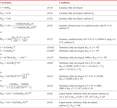
Table 8.4 summarizes the major correlations used for internal flow.

1. Laminar Flow, Fully Developed

Constant qs”: = = = = 4.36 f

D f

D

k D h Nu

k hD Nu

Constant Ts: = = = = 3.66 f

D f

D

k D h Nu

k hD

Nu

• Incompressible, constant property fluid assumed

• Axial conduction neglected

oExactly satisfied for constant qs”

(∂2T/∂x2 = 0)

oApproximated for constant Ts

• Evaluate k at Tm

• Valid at any ReD, Pr, or x since h is

independent of all these variables in fully developed laminar flow

oh depends only on conduit

diameter and fluid conductivity

oSee derivation in Section 8.4 in

textbook for constant qs” case

2. Laminar Flow, Entry Region

(a) Thermal Entry – Velocity profile is fully developed before heat flow (thermal boundary layer) occurs

! Valid for unheated initial lengths

of tube or large Pr fluids (δ >>δt)

Constant Ts: Hausen correlation

• Valid only for thermal entry lengths (i.e. fully developed velocity

boundary layer) or fluids with Pr ≥ 5 (δ "

µ

• All fluid properties evaluated at Tm=(Tm,in + Tm,out)/2

NOTE: This correlation may also be

written in terms of the Graetz number

Pr Re_D

D

x D

Gz = _"

(

)

(

)

[

]

04 . 0 1 Pr Re / 0668 . 0 66 . 3 D D D L D L D k D h Nu + + = =

[

]

(b) Combined Entry –The thermal and velocity boundary layers develop simultaneously in the entry region of the conduit

! NuD strongly dependent on

viscosity and thus Pr

! Flow is fully developed when

(x/D)/ReDPr = GzD ~ 0.05

Constant Ts: Baehr and Stephan:

[

]

(

)

(

)

1 67 . 0 33 . 0 Pr 432 . 2 tanh tanh 0499 . 0 7 . 1 264 . 2 tanh 66 . 3 − − − − ₊ + = D D D D D D Gz Gz Gz Gz Gz Nu

• Valid when Pr ≥ 0.1 and 0.0044 ≤

(

µ

µ

• All fluid properties evaluated at Tm

• NuD ≥ 3.66 (if you get a lower

number: use NuD = 3.66 since flow

would be primarily fully developed) • As Pr " ∞, denominator "1 – h

values within 3% of Hausen eq’n.

3. Turbulent Flow, Fully Developed

" fully developed velocity + thermal

Local correlations for constant Ts or

qs” for a smooth tube:

(a) If |Ts-Tm| is small - Dittus-Boelter n

D D

k hD

Nu = = 0.023Re0.8 Pr _(h

x = hL)

• Valid when 0.7 ≤ Pr ≤ 160, ReD ≥

10000, and L/D ≥ 10

• All fluid properties evaluated at Tm

• n=0.4 for fluid heating (Ts>Tm) or

n=0.3 for fluid cooling (Ts<Tm)

(b) If |Ts-Tm| is large – Sieder-Tate

14 . 0 8

.

0 1₃

Pr Re

027 .

0 _

  

 

= =

s D

D

k hD Nu

µ µ

(hx = hL)

• Valid when 0.7 ≤ Pr ≤ 16700, ReD ≥

10000, and L/D ≥ 10

• All fluid properties evaluated at Tm

except for

µ

For better accuracy over a larger Re range (3000 ≤ ReD ≤ 10000, including

transition region flow): Gnielinski

(

)(

)

(

)

(

)

. 12 1

Pr 1000 Re

8 /

67 . 0 5

. 0

−

+

−

= =

f f

k hD

Nu_D D

For a rough tube: higher f = higher h, but correlations become complex

Average correlations for constant Ts

or qs” tubes in turbulent regime:

Entry lengths are typically short If (L/D) < 60 " entry length is

typically significant, NuD > NuD,fd

₍

₎

fd D

D

D x

C Nu

Nu

+ =1

, C, m varies with inlet

If (L/D)>60 " entry length is not

significant, NuD~NuD,fd (<15% error)

f = friction factor " read from Moody

chart (f(ReD, e)) or, at low Re:

f~(0.79ln(ReD)-1.64)-2

E

MPIRICAL

C

ORRELATIONS

FOR

N

ON

-C

IRCULAR

T

UBES

For non-circular tubes, the circular tube results derived earlier can be applied when Re is evaluated using the hydraulic diameter instead of

diameter as the characteristic length.

P A

D c

h

4 =

Circular duct: A=πD2_{/4 and P=πD} " Dh = D

Square duct (side s): A=s2 _{and P=4s}

" Dh = s

Half-circle duct: A=πD2_{/8 and P=πD/2}

" Dh = D

Annular duct: A=π(Do2–Di2)/4

=π/4(Do–Di)(Do+Di) and P=π(Do+Di)

" Dh = Do - Di

Ac = flow cross-sectional area

P = perimeter of duct in contact with (i.e. “wetted by”) fluid

# Fully Developed Turbulent Flow

If ReDh > 2300 " use the hydraulic

diameter in the correlations presented above for Pr ≥ 0.7

# Fully Developed Laminar Flow

Sharp corners of square ducts alter flow so that circular duct correlations are not valid. See Table 8.1 for NuD

for both constant qs” and Ts.

EXAMPLE: Air flowing at 3x10-4 _kg/s

and 27o_{C enters a 1m long}

rectangular duct with a 4mm x 16 mm cross-sectional area. A uniform heat flux of 600 W/m2 _{is imposed on the}

duct surface. What is the

temperature of the air and the duct surface at the duct outlet?

Answer:

outlet air T = T

we need h -> convection heuristic

1. define object geometry:

2. define flow geometry: internal flow through duct

3. determine problem scope:

local h (surface T at outlet)

average h (overall fluid T)

4. define material properties:

for a duct - T of relevance for fluid

properties = T (mean temperature)

we can find mean outlet temperature using the fluid energy balance approaches

discussed

E

MPIRICAL

C

ORRELATIONS

FOR

C

ONCENTRIC

T

UBES

Fluid flows through an annulus formed by two concentric tubes (gray region)

Two convective surfaces exist in the gray area (inside tube and outside tube) with different h values. Thus two Nusselt numbers are used:

qi” = hi(Ts,i –Tm) and

i h i i

D

k D h Nu _, =

qo” = hi(Ts,o –Tm) and

o h o o

D

k D h Nu _, =

where Dh=Do-Di

Note: ki and ko are usually the same

Do

Di

• Fully Developed Turbulent Flow

! Dittus-Boelter equation evaluated

at D = Dh = Do - Di

n Dh

i o

h D

k D D

h k

hD

Nu = = ( − ) = 0.023Re0.8 Pr

Assumption: hi = ho (reasonably OK

for turbulent flow ONLY)

• Fully Developed Laminar Flow

(a) One surface at constant Ts/

One surface insulated

! Find Nuo and Nui for appropriate

Di/Do value in Table 8.2

(b) Both surfaces have constant qs”

! Find the influence coefficients

Nuoo, Nuii, θi*, and θo* for

appropriate Di/Do in Table 8.3

(

)

,

/

1 _{o i i}

ii i

D

q q

Nu Nu

θ

−

= _,

₍

₎

/

1 _{i o o}

oo o

D

q q

Nu Nu

θ

−

M

ICROCHANNEL

I

NTERNAL

F

LOW

We have already seen how conduction changes in thin gas films due to

interactions between gas molecules and the surrounding surfaces.

Similarly, convection in microchannels is influenced by both thermal and

momentum interactions between gas molecules and the solid walls.

In general: since ReD = ρu_µmD

Virtually all microscale internal flow is laminar (D<100

µ

For small D laminar flow,

NuD = hD/kf = 4.36 " h is typically

For gases, correlations previously described do not apply when

Dh/λmfp ≤ 100 (air: Dh < 10µm)

For liquids, correlations generally valid for Dh > 1µm (usually enough)

Both the thermal accommodation coefficient αt (conduction) and the

momentum accommodation

coefficient αp (advection) must be

considered in convection analysis.

s i

sc i

t

T T

T T

− −

=

α

and i s sc i

p

p p

p p

− −

=

α

i = gas molecule before surface collision

sc = gas molecule after surface collision

Specular reflection (speed unchanged, incidence=reflection angle) - αp = 0

Diffuse reflection (no preferred angle of reflection ,speed changed) - αp = 1

Air on all surfaces: 0.85 < αp < 1;

For laminar, fully developed flow in a circular tube and uniform qs”:

t D k hD Nu Γ + + − = = 48 6 11 48 2

ζ

ζ

where p

p Γ + Γ = 8 1 8 ζ (incompressible gas)

For two plates separated by a (Dh=2a)

( )

h D k hD Nu Γ + + − = = 70 3 2 6 17 140 2

ζ

ζ

where p

p Γ + Γ = 6 1 6 ζ (incompressible gas)

For both geometries (D = Dh):

     − = Γ D mfp p p p λ α α 2

γ = ratio of cp/cv , see values in Chapter 3

At large spacings, λmfp /Dh " 0 and

NuD=48/11 ~ 4.36 (consistent)

E

NHANCING

H

EAT

T

RANSFER

To enhance convective heat transfer: • Increase h

• Increase As

! Consider machining/ materials

cost, power requirements (∆P),

fluid properties (suspension?)

Another option: a coil introduces

centrifugal flow/ longitudinal vorticies according to coil diameter C and pipe diameter D (↑ h " see Equation 8.76)

(

)

s

conv hA T T

q = −

Coil Spring Twisted Tape

EXAMPLE: Two isothermal plates with dimensions 100x100mm are maintained at 350K by convective heat transfer to air flowing at 10m/s and with a temperature of 300K.