Land-use and land-cover change carbon emissions between 1901 and 2012 constrained by biomass observations

© Author(s) 2017. This work is distributed under the Creative Commons Attribution 3.0 License.

Land-use and land-cover change carbon emissions between 1901

and 2012 constrained by biomass observations

Wei Li1, Philippe Ciais1, Shushi Peng1,2, Chao Yue1, Yilong Wang1, Martin Thurner3, Sassan S. Saatchi4, Almut Arneth5, Valerio Avitabile6, Nuno Carvalhais7,8, Anna B. Harper9, Etsushi Kato10, Charles Koven11, Yi Y. Liu12, Julia E.M.S. Nabel13, Yude Pan14, Julia Pongratz13, Benjamin Poulter15, Thomas A. M. Pugh5,16, Maurizio Santoro17, Stephen Sitch18, Benjamin D. Stocker19,20, Nicolas Viovy1, Andy Wiltshire21,

Rasoul Yousefpour13,a, and Sönke Zaehle7

1_{Laboratoire des Sciences du Climat et de l’Environnement, LSCE/IPSL, CEA-CNRS-UVSQ,}

Université Paris-Saclay, 91191 Gif-sur-Yvette, France

2_{Sino-French Institute for Earth System Science, College of Urban and Environmental Sciences,}

Peking University, Beijing 100871, China

3_{Department of Environmental Science and Analytical Chemistry (ACES) and the Bolin Centre for Climate}

Research, Stockholm University, 106 91 Stockholm, Sweden

4_{Jet Propulsion Laboratory, California Institute of Technology, 4800 Oak Grove Drive, Pasadena, CA 91109, USA} 5_{Karlsruhe Institute of Technology, Institute of Meteorology and Climate Research – Atmospheric Environmental}

Research (IMK-IFU), Garmisch-Partenkirchen, Germany

6_{Centre for Geo-Information and Remote Sensing, Wageningen University & Research, Droevendaalsesteeg 3,}

6708PB Wageningen, the Netherlands

7_{Department for Biogeochemical Integration, Max-Planck-Institute for Biogeochemistry, Jena, Germany} 8_{CENSE, Departamento de Ciências e Engenharia do Ambiente, Faculdade de Ciências e Tecnologia,}

Universidade NOVA de Lisboa, Caparica, Portugal

9_{College of Engineering, Mathematics, and Physical Sciences, University of Exeter, Exeter, UK} 10_{Institute of Applied Energy, Minato, Tokyo 105-0003, Japan}

11_{Climate and Ecosystem Sciences Department, Lawrence Berkeley Lab, Berkeley, CA, USA} 12_{ARC Centre of Excellence for Climate Systems Science & Climate Change Research Centre,}

University of New South Wales, Sydney, New South Wales 2052, Australia

13_{Max Planck Institute for Meteorology, Hamburg, Germany} 14_{USDA Forest Service, Durham, New Hampshire, USA}

15_{Department of Ecology, Montana State University, Bozeman, MT 59717, USA}

16_{School of Geography, Earth & Environmental Science and Birmingham Institute of Forest Research,}

University of Birmingham, Birmingham, B15 2TT, UK

17_{GAMMA Remote Sensing, 3073 Gümligen, Switzerland}

18_{College of Life and Environmental Sciences, University of Exeter, Exeter, UK}

19_{Climate and Environmental Physics, and Oeschger Centre for Climate Change Research,}

University of Bern, Bern, Switzerland

20_{Imperial College London, Life Science Department, Silwood Park, Ascot, Berkshire SL5 7PY, UK} 21_{Met Office Hadley Centre, Exeter, Devon, EX1 3PB, UK}

a_{current address: Chair of Forestry Economics and Forest Planning, University of Freiburg, 79106 Freiburg, Germany}

Correspondence to:Wei Li (wei.li@lsce.ipsl.fr)

Received: 12 May 2017 – Discussion started: 2 June 2017

Abstract. The use of dynamic global vegetation models (DGVMs) to estimate CO2 emissions from land-use and

land-cover change (LULCC) offers a new window to ac-count for spatial and temporal details of emissions and for ecosystem processes affected by LULCC. One drawback of LULCC emissions from DGVMs, however, is lack of obser-vation constraint. Here, we propose a new method of using satellite- and inventory-based biomass observations to con-strain historical cumulative LULCC emissions (Ec_LUC) from an ensemble of nine DGVMs based on emerging relation-ships between simulated vegetation biomass and Ec_LUC. This method is applicable on the global and regional scale. The original DGVM estimates of Ec_LUCrange from 94 to 273 PgC during 1901–2012. After constraining by current biomass observations, we derive a best estimate of 155±50 PgC (1σ Gaussian error). The constrained LULCC emissions are higher than prior DGVM values in tropical regions but sig-nificantly lower in North America. Our emergent constraint approach independently verifies the median model estimate by biomass observations, giving support to the use of this es-timate in carbon budget assessments. The uncertainty in the constrained Ec_LUC is still relatively large because of the certainty in the biomass observations, and thus reduced un-certainty in addition to increased accuracy in biomass obser-vations in the future will help improve the constraint. This constraint method can also be applied to evaluate the impact of land-based mitigation activities.

1 Introduction

Carbon emissions from land-use and land-cover change (LULCC) are part of the human perturbation to the global carbon cycle (Houghton et al., 2012; Le Quéré et al., 2015) and started before the industrial era when fossil fuel CO2emissions appeared. Since 1850, estimated cumulative

LULCC emissions, Ec_LUC, have represented one-third of to-tal cumulative anthropogenic CO2emissions (Boden et al.,

2013; Houghton et al., 2012; Le Quéré et al., 2015). Annual LULCC emissions have been higher than those from fossil fuel burning until the 1930s (Boden et al., 2013; Houghton et al., 2012; Le Quéré et al., 2015) and today represent a smaller but persistent perturbation in the global carbon cycle. Unlike fossil fuel emissions, relative uncertainties in LULCC emis-sions are high due to the difficulty of assessing this flux from measurements. Some progress has been made to better quan-tify gross tropical deforestation emissions by combining spa-tial biomass data with satellite-derived maps delineating for-est cover loss (Harris et al., 2012). However, such spatially resolved data are not available beyond the last decade and provide only gross deforestation emissions, i.e., do not track the regrowth of secondary ecosystems or legacy soil carbon losses that can persist long after deforestation.

Bookkeeping models (Hansis et al., 2015; Houghton, 1999) based on historical LULCC area data and tabulated functions of carbon losses and gains are one approach to es-timating Ec_LUC, but they do not include the effects of environ-mental changes on carbon stocks before and after LULCC happens (Gasser and Ciais, 2013; Pongratz et al., 2014). The bookkeeping model of Houghton (1999) used for the annual update of the global carbon budget (Le Quéré et al., 2015) is based on regionally aggregated data and does not consider spatial differences in LULCC fluxes within a region. Alternatively, the estimated LULCC fluxes by dy-namic global vegetation models (DGVMs) account for spa-tial and temporal variations in carbon stock densities and land-cover change, as well as for delayed (“legacy”) carbon fluxes. In DGVMs, LULCC fluxes are related to environmen-tal conditions through simulated carbon cycle processes, i.e., net primary production (NPP) and respiration, resulting in changes in biomass and soil carbon stocks simulated with variable atmospheric CO2 concentration and climate. Yet,

LULCC emissions from DGVMs differ greatly, even when these models are prescribed with the same inputs of land-cover change data (such as time-variable areas of pasture and crops; Pitman et al., 2009). Several factors are responsible for differences in Ec_LUCamong DGVMs, including (1) different representations of processes that determine the carbon den-sities of vegetation and soils subject to land-use change; (2) using dynamic vegetation or prescribing a fixed vegetation distribution; and 3) the use of different rules assigning how natural vegetation types change to agricultural areas (Peng et al., 2017; Pitman et al., 2009; Reick et al., 2013).

Carbon initially stored in forest biomass contributes the predominant portion of the LULCC emissions after defor-estation (Hansis et al., 2015). Thus, an accurate represen-tation of the biomass carbon density exposed to LULCC is crucial to reduce uncertainties in DGVM-based Ec_LUC es-timates. Global biomass datasets based on inventories and satellites recently became available. These datasets (Table 1) provide the spatially distributed biomass carbon density on regional or global scales (Avitabile et al., 2016; Baccini et al., 2012; Carvalhais et al., 2014; Liu et al., 2015; Pan et al., 2011; Saatchi et al., 2011; Santoro et al., 2015; Thurner et al., 2014), but differ in terms of their coverage of aboveground or belowground biomass and whether they provide only forest biomass or biomass for all vegetation types.

Forest area change in PFT maps

Regression between cumulative LULCC emissions and initial biomass (in 1901) in models

Deforestation grid cells since 1901 in PFT maps

Cumulative LULCC emissions constrained by biomass observations

Present global biomass map based on observations

Regression between initial biomass (in 1901) and present biomass in models

Observation-based biomass in 1901 from Method A, B, C

Present biomass

Initial biomass

Initial biomass

LULCC emissions

Present biomass in deforestation grid cells using Method A, B, C

Figure 1.The framework of this study.

the DGVMs. The former set of regressions is used to extrap-olate present-day observation-based biomass (Table 1) to ini-tial biomass in the year 1901. The latter set of regressions is applied to provide an emerging constraint on Ec_LUCas a func-tion of initial biomass (Fig. 1). Using the Gaussian uncertain-ties associated with the observation-based biomass datasets and the uncertainties in the two regressions, the Gaussian er-rors in Ec_LUCcan be derived after applying the biomass con-straint.

2 Materials and methods

2.1 LULCC emissions and biomass from the DGVMs The DGVMs in TRENDY-v2 was used to conduct two sim-ulations (labeled S2 and S3) between 1860 (except JSBACH from 1850, Table 2) and 2012, with outputs quantifying LULCC emissions over the period 1901–2012 (Sitch et al., 2015). Both simulations are performed with changing cli-mate and CO2concentration, but one (called S3) has variable

LULCC maps based on Land-Use Harmonization (LUH) dataset (Hurtt et al., 2011; with an extension until 2012), and the other (called S2) has a time-invariant land-cover map representing the state in 1860. The difference in net biome production (NBP, the net carbon exchange between the bio-sphere and the atmobio-sphere) between these two simulations (S3 and S2) defines modeled LULCC emissions. This cal-culation of LULCC emissions by DGVMs includes the “lost sink capacity” (called “altered sink capacity” in Gasser and Ciais, 2013, and “the loss of additional sink capacity” in Pon-gratz et al., 2014) because simulated NBP in the S2 simu-lation without LULCC is a net sink over areas affected by LULCC in S3. For example, forests have larger carbon

stor-age and a slower turnover time than croplands and are thus expected to be carbon sinks when the atmospheric CO2level

increases. After deforestation to croplands, this sink capac-ity due to CO2 fertilization is lost. Modeled LULCC

emis-sions include the legacy emisemis-sions from soil carbon losses and emissions from wood and other products produced by LULCC, as far as the latter are included in the TRENDY-v2 models (Table 2). The DGVMs used in this study are CLM4.5 (Oleson et al., 2013), JSBACH (Reick et al., 2013), JULES3.2 (Best et al., 2011; Clark et al., 2011), LPJ (Sitch et al., 2003), LPJ-GUESS (Smith et al., 2001), LPX-Bern (Stocker et al., 2014), ORCHIDEE (Krinner et al., 2005), VISIT (Ito and Inatomi, 2012; Kato et al., 2013) and OCN (Zaehle and Friend, 2010). Each DGVM is described briefly in Table 2.

LULCC can either reduce or increase the biomass amount over time depending on the LULCC types. For example, forest clearing turns forest biomass into atmospheric CO2

T able 1. The dif ferent biomass datasets based on observ ations. The biomass information from the TREND Y -v2 project is also lis ted for comparison. Dataset Co v erage Resolution Biome type Abo v eground/belo wground Note Thurner et al. (2014) 30 ◦ N–80 ◦ N 0.01 ◦ forest abo v eground + belo wground Gro wing stock v olume from Santoro et al. (2015) Saatchi et al. (2011) 30 ◦ N–40 ◦ S 1 km forest abo v eground Carv alhais et al. (2014) global (without South Australia) 0.5 ◦ forest + herbaceous abo v eground + belo wground Mer ged map of Thurner et al. (2014) and Saatchi et al. (2011) Baccini et al. (2012) 23 ◦ N–23 ◦ S 500 m forest abo v eground Liu et al. (2015) global 0.25 de gree all abo v eground Calibration based on Saatchi et al. (2011) A vitabile et al. (2016) 30 ◦ N–40 ◦ S 1 km forest abo v eground Fusion of Saatchi et al. (2011) and Baccini et al. (2012) Santoro et al. (2015) 30 ◦ N + 0.01 ◦ forest abo v eground Sharing gro wing stock v olume with Thurner et al. (2014) P an et al. (2011) global re gional forest abo v eground + belo wground Based on F A O data TREND Y -v2 global 1 ◦ all abo v eground + belo wground China region 0 5 10 North America 0 5 10 South and Central America Western Europe Tropical Africa 1910 1960 0 5 10 The former Soviet Union South and Southeast Asia 1910 1960 Pacific developed region

1910 1960 2010 North Africa and Middle East

CLM4.5 JSBACH JULES3.2 LPJ LPJ-GUESS LPX-Bern ORCHIDEE VISIT OCN Fo re s t a re a ( m ill io n k m ) 2 Year

Figure 2.Temporal change in forest area from TRENDY-v2 models

in each of the nine regions. Differences between models arise from their specific vegetation maps and rules through which natural PFTs are chosen to give land to agriculture.

LULCC-affected grid cells in all models. For the same rea-sons, the forest areas and the LULCC types are also different among models.

In this study, we adopted the “deforestation grid cells” in their corresponding PFT maps as a criterion to locate the LULCC-affected grid cells from DGVM outputs. Thus we used the PFT maps from each model to first calculate the temporal change in forest area (total area of all forest PFTs) during 1901–2012 and then selected the grid cells that ex-perienced deforestation by comparing the forest area maps between 1901 and 2012 (net deforestation). This procedure produces a good approximation given the continuously de-creasing trend of forest area in LULCC hotspot regions like South and Central America (Fig. 2). We also tested an alter-native method to determine the LULCC-affected grid cells in TRENDY model outputs; i.e., PFT maps were compared year by year during 1901–2012, and grid cells with deforesta-tion were selected (gross deforestadeforesta-tion). This method tends to give a greater number of LULCC-affected grid cells, reduc-ing the goodness of fit in the regression between the biomass in 1901 and Ec_LUCduring 1901–2012 (Figs. S1 and S2 in the Supplement). Therefore, the method of gross deforestation is not used for further analyses.

tran-T able 2. Description of TREND Y model setups used in this study . Model PFT number Allocati on rules of changes in agriculture area Spatial resolution dynamic vegetation acti

sitions involving pairs of non-forest PFTs in the selected grid cells.

In each model, only biomass in deforestation grid cells is considered. Biomass in the year 1901 is thereby defined as

initialbiomass, and biomass averaged during 2000–2012 is defined as present biomass. An ordinary least squares lin-ear regression is performed with the outputs of all models between initial biomass and Ec_LUC from 1901 to 2012 and between the initial and the present biomass on both global and regional scales. Our division of nine regions in the world (Fig. 2) for estimating LULCC fluxes is the same as in Houghton et al. (1999).

2.2 Observation-based biomass datasets

Several biomass datasets (Avitabile et al., 2016; Baccini et al., 2012; Carvalhais et al., 2014; Liu et al., 2015; Pan et al., 2011; Saatchi et al., 2011; Santoro et al., 2015; Thurner et al., 2014) based on inventories and remote sensing can po-tentially be used to constrain Ec_LUC through the set of re-gressions from DGVMs. However, these biomass datasets cover different parts of biomass (aboveground, belowground or total) and different regions (tropics, Northern Hemisphere or the globe) at different spatial resolutions (Table 1). We choose the global grid-based biomass dataset from Carval-hais et al. (2014) to derive an observational constraint that re-sults in a best estimate of Ec_LUC. This map merges the North-ern Hemisphere biomass dataset from Thurner et al. (2014) and the tropical biomass dataset from Saatchi et al. (2011). An advantage of this map is its consistency in biomass terms with the outputs of TRENDY models because it docu-ments aboveground+belowground and forest+herbaceous biomass (Tables 1, 2). Three other biomass maps are used as alternative datasets for sensitivity tests: (1) the global biomass map from the GEOCARBON project, a merged product of the biomass datasets in the Northern Hemisphere (Santoro et al., 2015) and tropics (Avitabile et al., 2016); (2) regional biomass estimates from Pan et al. (2011) based on forest inventory data; and (3) the biomass map from Liu et al. (2015) derived from satellite vegetation optical depth. The GEOCARBON (Avitabile et al., 2016; Santoro et al., 2015) and Liu et al. (2015) datasets that only provide aboveground biomass were extended to total forest biomass using the con-version factors for the nine regions (Liu et al., 2015). The global biomass maps from GEOCARBON (Avitabile et al., 2016; Santoro et al., 2015) and Pan et al. (2011) are only for forest (Table 1), and we do not add the herbaceous biomass to these two datasets because the global herbaceous biomass only accounts for about 3 % of the global total biomass (Car-valhais et al., 2014). Note that the uncertainties in the cor-responding constrained results using these three alternative datasets do not include (1) the uncertainties in converting aboveground biomass to the total of aboveground and below-ground biomass for the datasets from Liu et al. (2015) and GEOCARBON (Avitabile et al., 2016; Santoro et al., 2015)

or (2) the uncertainties in ignoring non-woody biomass in the datasets from GEOCARBON (Avitabile et al., 2016; Santoro et al., 2015) and Pan et al. (2011). The biomass maps of Car-valhais et al. (2014), GEOCARBON (Avitabile et al., 2016; Santoro et al., 2015) and Liu et al. (2015) with different spa-tial resolutions were aggregated to a 1◦×1◦resolution be-fore selecting the debe-forestation grid cells.

2.3 Methods to identify grid cells subject to past deforestation in biomass datasets

It is not practical to use PFT maps from DGVMs to de-fine deforestation grid cells in the observation-based biomass datasets because PFT maps and forest area change since 1901 differ across DGVMs. Instead, we diagnosed defor-estation grid cells in the biomass maps using three harmo-nized methods (Method A, Method B and Method C). All the methods are based on the reconstructed historical agri-cultural area from the History Database of the Global En-vironment (HYDE v3.1; Klein Goldewijk et al., 2011) but with different hypotheses regarding how agricultural expan-sion has affected forests. These harmonized methods are rep-resentative of the different rules for assigning LULCC data to natural vegetation types in DGVMs. Method-A assumes that the increase in cropland area in a grid cell between 1901 and 2012 is taken from forest; Method B assumes that the increase in cropland and pasture is taken proportionally from all natural vegetation types; and Method C (like the “BM3” scenario in Peng et al., 2017) assumes that the increase in cropland and pasture is first taken from forest and then from natural grassland if no more forest area is available and that the regional forest area change is set to match the histori-cal forest reconstruction from Houghton (2003). Because the biomass distribution in Pan et al. (2011) is given as regional mean values and not resolved on a grid cell basis, it is im-possible to select deforestation grid cells directly from this dataset using the above methods. Therefore, for each region, we calculated the ratios of biomass in deforestation grid cells according to Method A, Method B and Method C to the total biomass in all grid cells in each of the other three biomass datasets (Carvalhais et al., 2014; GEOCARBON, Avitabile et al., 2016; Santoro et al., 2015; Liu et al., 2015). For each method (Method A, B and C), the three ratios correspond-ing to the three biomass datasets were further averaged in each region. The total biomass amount from Pan et al. (2011) in each region was multiplied by the average ratio to derive the biomass equivalent to using Method A, Method B and Method C for the dataset from Pan et al. (2011).

1901 in the selected grid cells using these three methods is higher than using PFT maps, but the Ec_LUCare lower, reflect-ing a lower representativeness of the deforestation grid cells using these three methods for DGVM outputs (Fig. S1). As a consequence, a weaker goodness of regression fit was found between Ec_LUCand initial biomass (Fig. S2).

2.4 Uncertainties in constrained LULCC emissions

The biomass from Method A, Method B and Method C ob-tained from each dataset is extrapolated into biomass for the year 1901 using the regression between initial biomass and present biomass modeled by the DGVMs. This biomass in 1901 is then applied in the regression between modeled Ec_LUCand modeled initial biomass among different DGVMs to calculate constrained Ec_LUC. In this emerging constraint approach (Fig. 1), the uncertainties in constrained Ec_LUC are a function of the uncertainties in the observed biomass datasets, the linear regression goodness of fit for the two re-gressions (rere-gressions between Ec_LUCand the initial biomass and between the initial and present biomass) and the slopes of the regressions. The uncertainty in constrained LULCC emissions is calculated as in Stegehuis et al. (2013):

σLULCC=

q α2_σ2

initial_biomass+σ

2

res_LULCC , (1)

σinitial_biomass=

q β2_σ2

present_biomass+σ

2

res_biomass , (2)

whereσLULCC,σinitial_biomass andσpresent_biomass are the

un-certainties in constrained Ec_LUC, the uncertainty in initial biomass and the uncertainty in present biomass; α and

σres_LULCC represent the slope and the standard deviation of

the residuals from the linear regression fit between Ec_LUCand initial biomass, andβandσres_biomassrepresent the slope and

standard deviation of the residuals from the linear regression between initial biomass and present biomass.

2.5 Two supplementary methods to constrain Ec_LUC using biomass observations

We also tested two supplementary methods to constrain Ec_LUC: first, Method S1 using the regression between Ec_LUC and present-day biomass from TRENDY models rather than extrapolating present biomass to biomass in 1901, and then Method S2 using 1B (biomass difference between present biomass and biomass in 1901 derived from the model simu-lations) instead of a regression between biomass in 1901 and present-day biomass to extrapolate the observation-based biomass in 1901. In Method S1, the uncertainties in the biomass observations and in the regression between Ec_LUC and present biomass from the models are used to calculate the uncertainties in the constrained Ec_LUC. In Method S2, the uncertainties in the biomass observations and the standard deviation of1B among the models are used.

10 20 30 40 0

5 10 15 20

y = 0.37x+1.48 r = 0.262

China region

10 30 50 70 0

20 40

y = 0.42x+0.16 r = 0.702

North America 100 150 200 250 300 10

30 50 70 90

y = 0.21x+12.09 r = 0.612

South and Central America

2 6 10 14 0

2 4 6 8

y = 0.13x+2.45 r = 0.092

Western Europe 20 60 100 140 0

20 40 60

y = 0.37x-0.94 r = 0.762

Tropical Africa

10 30 50 70 90 0

10 20 30

y = 0.29x+2.57 r = 0.902

The former Soviet Union

20 50 80 110 140 0

20 40 60

y = 0.36x-2.02 r = 0.582

South and Southeast Asia

5 15 25 35 10

0 10 20

y = 0.44x-4.72 r = 0.492

Pacific developed region

0 2 4 6 2

2 6

y = 0.63x-0.30 r2_{= 0.48}

North Africa and Middle East

CLM4.5 JSBACH JULES3.2 LPJ LPJ-GUESS LPX-Bern ORCHIDEE VISIT OCN

300 500 700 900 0

50 100 150 200 250 300

y = 0.31x+11.80 r = 0.662

Globe

Cumulative LULCC emissions (Pg C)

Biomass in 1901 (Pg C)

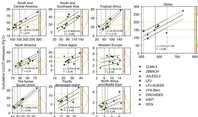
Figure 3.Relationship between biomass in 1901 and cumulative land-use and land-cover change (LULCC) emissions during 1901–2012

across the nine TRENDY-v2 models. The black solid line is the linear regression line. The vertical green solid line indicates the reconstructed biomass in 1901 from Carvalhais et al. (2014) by applying Method A (the increase in cropland in HYDE v3.1 data from forest; see Figs. S4 and S5 for the results of Method B and Method C) to define deforestation grid cells. The orange solid horizontal line indicates the cumulative

LULCC emissions constrained by reconstructed biomass in 1901. Dashed lines represent 1σuncertainties. The probability density function

of the constrained cumulative LULCC emissions is shown on the right.

3 Results

3.1 Forest area change and cumulative LULCC emissions in DGVMs

As expected, a general decrease in forest area is found be-tween 1901 and 2012, especially in regions subject to ex-tensive deforestation over the last decades, namely South and Central America, South and Southeast Asia and tropi-cal Africa (Fig. 2), which is in support of our methods of defining deforestation grid cells, although the forest area in some regions differs substantially across DGVMs. Differ-ences in forest area are large in tropical Africa, North Amer-ica and the former Soviet Union, while they are smaller in South and Central America and South and Southeast Asia (Fig. 2). There are several reasons for these differences in forest area: (1) the models have different initial distributions of PFTs (the TRENDY-v2 protocol only prescribed the same initial area of natural vegetation, but did not specify the PFTs that compose natural vegetation); (2) some models consider only net LULCC, but others have gross LULCC including some sub-grid transitions (Table 2; see a comparison using the JSBACH model; Wilkenskjeld et al., 2014); (3) and the models have different treatments for changing pasture areas (either proportional from natural vegetation or preferential from natural grasslands). In North America, the China re-gion and Western Europe, the forest area decreased in the first

half of the 20th century and then increased in recent decades. Yet, the magnitude of the increase is smaller than that of the previous decrease in these regions, and the global average is net forest loss between 1901 and 2012 (ranging from 2.3 to 16.8 Mkm2across the nine models).

Ec_LUC from the nine DGVMs between 1901 and 2012 range from 1.7 PgC (−0.6 to 6.0; median and range are pos-itive, indicating a net cumulative flux to the atmosphere) in North Africa and the Middle East to 42.6 PgC (33.5 to 81.4) in South and Central America, resulting in a global total of 148 PgC (94 to 273; Table 3). Tropical Africa and South and Southeast Asia have the second-largest Ec_LUCof 21.8 (15.8 to 57.8) and 21.8 PgC (9.6 to 46.6), respectively. Although af-forestation and reaf-forestation occurred in North America after around 1960 and in China after 2000 (Fig. 2), Ec_LUCin these two regions have been positive since 1901, with median val-ues of 19.9 and 10.7 PgC, respectively (Table 3).

3.2 Relationship between cumulative LULCC emissions and initial biomass

in-creasing forest area (Fig. 2), the correlation between initial biomass and Ec_LUCis small in Western Europe (Fig. 3). The slopes of the relationships between Ec_LUCand initial biomass shown in Fig. 3 range from 0.13 PgC PgC−1in Western Eu-rope to 0.63 PgC PgC−1in North Africa and the Middle East. In tropical regions with intensive LULCC, the slope is simi-lar between South and Southeast Asia (0.36 PgC PgC−1) and tropical Africa (0.37 PgC PgC−1), but lower in South and Central America (0.21 PgC PgC−1). These slopes reflect the sensitivity of cumulative carbon loss to initial biomass car-bon stock. They are mainly influenced by the fraction of de-forested area relative to the initial forest area in each region, which explains 46 % of the variations in the slopes across regions (Fig. S3). Differences in biomass density across regions and in the use of gross or net transitions among DGVMs (Table 2) also contribute to variations in slopes.

3.3 Cumulative LULCC emissions constrained by present-day biomass observations

There is also a strong positive relationship between initial biomass in 1901 and present-day biomass in grid cells that have experienced deforestation (Fig. 4). The r2 of this re-gression is higher than 0.92 in most regions, except in North America and the China region (0.89 and 0.76, respectively). The regression between present-day and initial biomass was applied to extrapolate current observation-based biomass back to the year 1901. The extrapolated biomass in 1901 is higher than that in the present day, mainly due to a larger for-est area, although it is difficult to discriminate other effects, such as CO2fertilization, that might have increased biomass

between 1901 and 2012.

Using the chain of emerging constraints between present-day and initial biomass (Fig. 4) and between Ec_LUCand ini-tial biomass (Fig. 3), with all uncertainties being propagated (Eqs. 1 and 2), we were able to constrain Ec_LUCduring 1901– 2012 by biomass observations (Figs. 3, S4, S5, Table 3). The Ec_LUCvalue constrained by the biomass dataset of Carvalhais et al. (2014) is 155±50 PgC (mean and 1σ Gaussian error) and this estimate is robust to the choice of the methods to de-fine deforestation grid cells in biomass datasets (constrained Ec_LUC=152±49, 154±50 and 159±51 PgC for Method A, Method B and Method C, respectively). The difference be-tween the global constrained Ec_LUCand the median value of original Ec_LUC(148 PgC) from TRENDY DGVMs is not sig-nificant, suggesting that the median model estimate is inde-pendently verified by biomass observations. Still, some mod-els that are inconsistent with the observations can be identi-fied (Fig. 3).

The uncertainties reported in our constrained estimate of Ec_LUCinclude uncertainties in the biomass observations and in the scatter of the two regressions (Figs. 3, 4) used to struct the emerging constraint. The uncertainties in the con-strained Ec_LUC are still relatively large, resulting from the large uncertainties in the biomass observations. However, it

should be noted that we summed the biomass uncertainty in each deforestation grid cell to give the regional biomass uncertainty, which gives a maximum uncertainty with a po-tential assumption that the uncertainties in all grid cells are fully correlated. In reality, the regional biomass uncertainty should be lower, thus leading to lower uncertainty in con-strained Ec_LUC. However, it is difficult to estimate the error correlations of observation-based biomass between different grid cells at this stage.

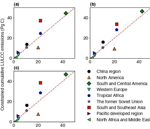
Although the constrained global Ec_LUCvalue is only 7 PgC higher than the median of the original DGVM ensemble (Ta-ble 3), larger differences can be found on a regional scale (Fig. 5). Constrained Ec_LUCestimates are higher than the orig-inal modeled values in South and Southeast Asia, tropical Africa and South and Central America (Table 3). For exam-ple, the constrained Ec_LUCvalue is 37.2±14.4 PgC in South and Southeast Asia compared to the original TRENDY me-dian value of 21.8 PgC (range of 9.6 to 46.6 PgC) for that re-gion. The constrained emissions are also higher in the China region and the Pacific developed region compared to the prior median value (see Table 3). A significantly large re-duction in Ec_LUCthrough the emerging constraint is found in North America because of the lower biomass amount from observation-based datasets than from DGVMs. The original median Ec_LUC value of that region is 19.9 PgC (range of 8.6 to 40.8 PgC), while the constrained result is 10.8±7.1 PgC. Constrained Ec_LUC are also lower than original estimates in Western Europe, North Africa and the Middle East, although their contributions to the global total emissions are very small (Table 3).

uncer-10 20 30 40 10

20 30 40

y = 0.86x+10.10 r = 0.762

China region

25 50 75 20

40 60 80

y = 1.07x+3.25 r = 0.892

North America 100 200 300 100

200 300

y = 0.92x+33.85 r = 0.922

South and Central America

5 10 15

5 10 15

y = 1.03x+1.27 r = 0.942

Western Europe 20 60 100 140 20

60 100 140

y = 1.23x-1.83 r = 0.972

Tropical Africa

0 50 100

0 50 100

y = 0.95x+3.84 r = 0.952

The former Soviet Union

50 100 50

100

y = 1.12x+2.12 r = 0.962

South and Southeast Asia

20 40

10 20 30 40

y = 1.07x+0.18 r = 0.942

Pacific developed region

0.0 2.5 5.0 0

2 4 6

y = 1.49x-0.21 r = 0.962

North Africa and Middle East

CLM4.5 JSBACH JULES3.2 LPJ LPJ-GUESS LPX-Bern ORCHIDEE VISIT OCN

Biomass in 1901 (Pg C)

Present biomass (Pg C)

Figure 4.The relationship between initial biomass in 1901 and present biomass (average of biomass from 2000 to 2012) across the

TRENDY-v2 models for each region. Note that both biomass in 1901 and present biomass are from TRENDY models, not the observations. Dashed

line is the 1:1 line.

tainty, which is about one-third of the mean biomass at the global level (Carvalhais et al., 2014).

The global constrained Ec_LUCvalue obtained by using the two supplementary methods is almost identical to that from our original method in Fig. 1 (see an example in Fig. S6). The difference in Ec_LUCbetween the supplementary and orig-inal methods at the global level is < 1 % for all biomass ob-servation datasets (Carvalhais et al., 2014; Liu et al., 2015; GEOCARBON, Avitabile et al., 2016; Santoro et al., 2015; Pan et al., 2011) and all methods to select LULCC grid cells (Method A, B and C). This suggests that our constrained re-sults are very robust. The change in the uncertainty in global constrained Ec_LUC is also very small (< 2 %) because most of the uncertainties are from the biomass observations (see Discussion) and the regression between Ec_LUC and biomass (see r2 in Fig. 3), rather than from converting present-day biomass to biomass in 1901 (see r2 in Fig. 4). The differ-ence in regional Ec_LUCbetween different constraint methods is relatively larger (12 % on average), but the difference re-mains very small in tropical regions (∼1 %). However, we note that the results from the two supplementary methods (Method S1 and S2) should be cautiously treated. First, be-cause Ec_LUCare related to the biomass that has been affected since the start of the land-use perturbation, only biomass in 1901 (rather than that left out of land use in the 2000s)

in LULCC-affected grid cells is logically related to histori-cal Ec_LUC. Thus, converting present-day biomass to biomass in 1901 (the original method; Fig. 1) is a more direct and process-justified approach compared to regressing present-day biomass versus Ec_LUC (Method S1), which is not justi-fied by a logical mechanism. Second, using1B in Method S2 is not a perfect solution to extrapolate biomass in 1901 from present-day biomass because the change in biomass is not solely impacted by land-use change. The interactions be-tween biomass and climate conditions, disturbances and nu-trient limitation are also very important in DGVMs. For ex-ample, historical LULCC may reduce biomass over LULCC-affected regions by replacing forests with croplands. On the contrary, the CO2fertilization effects may increase biomass

0 20 40 0

20 40

(a)

0 20 40 0

20 40

(b)

0 20 40 0

20 40

(c)

China region North America

South and Central America Western Europe Tropical Africa The former Soviet Union South and Southeast Asia Pacific developed region North Africa and Middle East

Constrained cumulative LULCC emissions (Pg C)

Original cumulative LULCC emissions (Pg C)

Figure 5.Comparisons between the original TRENDY land-use and

land-cover change (LULCC) emissions and the cumulative LULCC emissions constrained by the biomass dataset from Carvalhais et

al. (2014). Panels (a),(b)and(c)are the results from Method A,

Method B and Method C, respectively. The original TRENDY emis-sions are shown as the median value of all models. Dashed line is

the 1:1 line.

4 Discussion

Our approach to constraining Ec_LUC from an ensemble of DGVMs provides a best estimate that is between those from two bookkeeping models (∼130 PgC from Houghton et al., 2012, and 212 PgC for the default dataset from Hansis et al., 2015). Although the bookkeeping model from Hansis et al. (2015) was driven by the same agricultural land-use maps as the TRENDY models (the model of Houghton et al., 2012, uses FRA/FAO data), the Ec_LUCvalue from Han-sis et al. (2015) is different from that constrained from the DGVMs. Differences in estimates between DGVMs and bookkeeping models have been attributed to different defini-tions of LULCC emissions (Pongratz et al., 2014; Stocker and Joos, 2015). Indeed, LULCC emissions from DGVM simulations in TRENDY include the “missed sink capacity in the deforested area” (Gasser and Ciais, 2013; Pongratz et al., 2014), and so, all else being equal, should simulate higher emissions than bookkeeping models, which do not include this term. However, bookkeeping models take for-est degradation into account, while this process is ignored in DGVMs. Bookkeeping models also represent shifting cul-tivation (resulting in larger sub-grid-scale gross land transi-tions as opposed to net transitransi-tions) and wood harvest; these are processes that are accounted for in only a subset of the TRENDY models (see Table 2). In addition to different driv-ing LULCC area data, differences between the two book-keeping models were discussed by Hansis et al. (2015); for

Original TRENDY

Carvalhais et al. Liu et al. GEOCARBON Pan et al.

0 50 100 150 200 250

Cumulative LULCC emissions (Pg C)

Method A Method B Method C

All methods All methods Method A Method B Method C All methods Method A Method B Method C All methods Method A Method B Method C

Figure 6.The global cumulative land-use and land-cover change

(LULCC) emissions during 1901–2012 from original TRENDY models and from the estimates constrained by different biomass datasets with different methods to define deforestation grid cells. “All methods” represents the ensemble mean and uncertainty in the constrained results from Method A, Method B and Method C for each biomass dataset. The whisker–box plot represents the mini-mum and maximini-mum values, 25th and 75th percentiles and the me-dian value of original TRENDY models. In the bar plot for the

con-strained estimates, the red line represents the 1σ Gaussian errors;

the black ticks represent the 25th and 75th percentiles.

example, Houghton et al. (2012) assumed a preferential al-location of pastures on natural grasslands, while Hansis et al. (2015) assumed a proportional allocation of both cropland and pasture on all available natural vegetation types.

We are aware that our truncated diagnostic of a set of de-forestation grid cells, instead of grid cells affected by all LULCC types, is an underestimate of the total area subject to LULCC because we ignore grid cells that experienced land-use transitions between non-forest vegetation only (e.g., only conversions from grasslands to cropland happening in a grid cell). However, the conversion of forest to croplands and pasture dominates the total net LULCC flux (Houghton, 2003, 2010), while the contribution of transitions between non-forest vegetation and agriculture to Ec_LUC is compara-tively small (Fig. S1). In fact, the annual LULCC emission from deforestation was estimated to be 2.2 PgC yr−1during the 1990s, and the total emissions from other activities (e.g., afforestation, reforestation, non-forest transitions) are nearly neutral (Houghton, 2003).

nu-trient limitation on biomass. Despite these uncertainties, the high coefficient of determination in the regression increases our confidence in the biomass extrapolation to 1901. For a given biomass dataset, the choice of a method for defining deforestation grid cells (Method A, Method B and Method C) has a very small influence on our results (Table 3).

LULCC carbon emissions are influenced not only by changes in biomass, but also by how these are prescribed in the model to influence posterior changes in detrital and soil organic carbon pools. However, LULCC emissions are domi-nated by changes in biomass. For example, LULCC results in a net carbon loss of 110 PgC in biomass during 1850–1990, accounting for 89 % of the total Ec_LUC(Houghton, 1999). The soil carbon changes after LULCC is also indirectly impacted by initial biomass, since the dead roots and remaining above-ground debris turn into soil organic carbon after land clear-ing, which takes longer to return into the atmosphere. In addi-tion, it is not necessary to account for all factors when apply-ing an emergent constraint approach (e.g., Cox et al., 2013; Kwiatkowski et al., 2017; Wenzel et al., 2016). The regres-sion between Ec_LUCand biomass in 1901 in the models in our study is satisfying (e.g.,r2=0.66 on a global scale; Fig. 3) to constrain Ec_LUCthrough biomass observations.

The required model outputs for carbon stocks and fluxes in the TRENDY project are not PFT specific; only the mean PFT-mixed variables in each grid cell are required. Such an aggregation prevents a rigorous separation of biomass be-tween forest and other biomes in each grid cell. It was thus impossible for us to calculate individual contributions of dif-ferent LULCC types to the overall LULCC emissions, which induces uncertainties when matching model results with ob-served forest biomass distributions (e.g., only forest biomass in datasets from GEOCARBON; Avitabile et al., 2016; San-toro et al., 2015; Pan et al., 2011). Therefore, we suggest that the next generation of DGVM comparisons report PFT-specific carbon stock and fluxes, and other model intercom-parison exercises should follow suit. The approach of us-ing multiple biomass observation datasets to constrain the LULCC emissions could also be applied in other model-ing projects, such as Coupled Model Intercomparison Project Phase 5 (CMIP5) and CMIP6.

Currently, the uncertainties in the satellite-based biomass datasets are relatively large (e.g., 38 % on average in the trop-ics at the pixel level (< 1 km); Saatchi et al., 2011). This in-troduces uncertainties in the constrained cumulative LULCC emissions, depending on the forest types and biomass range. For example, on average on the global scale, the uncertainty in the resolution of DGVM grid cells (0.5◦_×0.5◦_{) is about}

one-third of the mean biomass (Carvalhais et al., 2014) and the relative uncertainty is smaller for high biomass areas in the tropics (Avitabile et al., 2016; Saatchi et al., 2011).

The main sources of uncertainties in satellite-based biomass datasets depend on the specific product, the spa-tial resolution of the datasets and the methodology used to validate the data. For instance, in the case of radar remote

sensing used for biomass mapping in Northern Hemisphere boreal and temperate forests, the uncertainty is largely due to the sensitivity of the signal to properties other than vegetation structure (e.g., moisture), the influence of non-forest vegeta-tion on the signal (especially in fragmented landscapes; San-toro et al., 2015) and uncertainties in the additional datasets (allometric databases, land cover) used for the conversion of satellite measurements to biomass estimates (Thurner et al., 2014). At the pixel level and modeling grid cells, uncertain-ties may also be strongly influenced by the quality and size of the inventory data used for validation and the significant mismatch between pixel area and the plot data, as well as the difference between the dates of satellite and ground observa-tions (Saatchi et al., 2015, 2011; Thurner et al., 2014).

Moreover, the satellite-derived biomass datasets used in this study represent different dates. The tropical biomass products represent the circa 2000 status of forests, whereas the boreal and temperate biomass maps are based on space-borne radar data from the year 2010. These differences in the date of observations introduce additional uncertainty in the biomass estimates due to changes in forest cover from the disturbance, recovery and land-use activities (Hurtt et al., 2011) occurring annually and regionally.

However, in boreal, temperate and in tropical regions, the estimated relative uncertainties were lowest in high biomass areas (Avitabile et al., 2016; Thurner et al., 2014), which dominate the contribution to our results. Moreover, the rel-atively high accuracy of biomass datasets when aggregated to modeling grid cells from higher-resolution maps (< 1 km; Saatchiet al., 2011; Thurner et al., 2014) suggests that the biomass datasets implemented in our study provide a realis-tic representation of carbon stocks to constrain the historical cumulative LULCC emissions from vegetation.

5 Conclusions

mod-eled variables (an observable and an unknown one) with ac-tual observations of the observable variable. Thus, our study shows (1) that there is a heuristic relationship between initial biomass and Ec_LUCamong different models, (2) that available biomass observation data independently confirm the median of modeled emission estimates and (3) that more accurate biomass data in the future would allow some of the mod-eled estimates of emissions to be falsified. Although the un-certainties in current observation-based biomass datasets are relatively high, as more accessible and accurate observation data become available, many data-driven opportunities are being created to improve the accuracy of DGVM predictions.

Data availability. Different biomass datasets used in this study

can be downloaded based on information in their original publica-tions. Specifically, the biomass dataset of Carvalhais et al. (2014) can be downloaded from MPI BGI Data Portal: https://www. bgc-jena.mpg.de/geodb/projects/Home.php; The biomass dataset of Liu et al. (2015) can be downloaded from http://www. wenfo.org/wald/global-biomass/; The biomass dataset of GEO-CARBON (Avitabile et al., 2016; Santoro et al., 2015) can be downloaded from http://www.wur.nl/en/Expertise-Services/Chair-groups/Environmental-Sciences/; The regional biomass of Pan et al. (2011) can be found in Table 2 in their paper. The outputs (biomass-constrained cumulative LULCC emissions) of this study are provided in Table 3.

The Supplement related to this article is available online at https://doi.org/10.5194/bg-14-5053-2017-supplement.

Competing interests. The authors declare that they have no conflict

of interest.

Acknowledgements. Wei Li, Chao Yue, Thomas A. M. Pugh and

Almut Arneth were supported by the project LUC4C funded by the European Commission (grant no. 603542). Philippe Ciais and Shushi Peng acknowledge support from the European Re-search Council through Synergy grant ERC-2013-SyG-610028 “IMBALANCE-P”. Julia Pongratz, Julia E. M. S. Nabel and Rasoul Yousefpour were supported by the German Research Foundation’s Emmy Noether Program (PO 1751/1-1). Ben-jamin D. Stocker was supported by the Swiss National Science Foundation and FP7 funding through project EMBRACE (282672). Anna B. Harper was supported by the UK Natural Environment Research Council Joint Weather and Climate Research Programme. Martin Thurner acknowledges funding from the Vetenskapsrådet (grant no. 621-2014-4266 of the Swedish Research Council). The biomass maps and model outputs can be freely accessed by following the instructions in the original publications. All the biomass-constrained LULCC emission data can be freely obtained from Wei Li (email: wei.li@lsce.ipsl.fr).

Edited by: Christopher A. Williams Reviewed by: two anonymous referees

References

Avitabile, V., Herold, M., Heuvelink, G. B. M., Lewis, S. L., Phillips, O. L., Asner, G. P., Armston, J., Ashton, P. S., Banin, L. F., Bayol, N., Berry, N. J., Boeckx, P., de Jong, B. H. J., De-Vries, B., Girardin, C. A. J., Kearsley, E., Lindsell, J. A., Lopez-Gonzalez, G., Lucas, R., Malhi, Y., Morel, A., Mitchard, E. T. A., Nagy, L., Qie, L., Quinones, M. J., Ryan, C. M., Ferry, S. J. W., Sunderland, T., Laurin, G. V., Gatti, R. C., Valentini, R., Verbeeck, H., Wijaya, A., Willcock, S., Asthon, P., Banin, L. F., Bayol, N., Berry, N. J., Boeckx, P., de Jong, B. H. J., DeVries, B., Girardin, C. A. J., Kearsley, E., Lindsell, J. A., Lopez-Gonzalez, G., Lucas, R., Malhi, Y., Morel, A., Mitchard, E. T. A., Nagy, L., Qie, L., Quinones, M. J., Ryan, C. M., Slik, F., Sunderland, T., Vaglio Laurin, G., Valentini, R., Verbeeck, H., Wijaya, A., and Willcock, S.: An integrated pan-tropical biomass map using multiple reference datasets, Glob. Change Biol., 22, 1406–1420, https://doi.org/10.1111/gcb.13139, 2016.

Baccini, A., Goetz, S. J., Walker, W. S., Laporte, N. T., Sun, M., Sulla-Menashe, D., Hackler, J., Beck, P. S. A., Dubayah, R., Friedl, M. A., Samanta, S., and Houghton, R. A.: Estimated carbon dioxide emissions from tropical deforestation improved by carbon-density maps, Nature Climate Change, 2, 182–185, https://doi.org/10.1038/nclimate1354, 2012.

Best, M. J., Pryor, M., Clark, D. B., Rooney, G. G., Essery, R. . L. H., Ménard, C. B., Edwards, J. M., Hendry, M. A., Porson, A., Gedney, N., Mercado, L. M., Sitch, S., Blyth, E., Boucher, O., Cox, P. M., Grimmond, C. S. B., and Harding, R. J.: The Joint UK Land Environment Simulator (JULES), model description – Part 1: Energy and water fluxes, Geosci. Model Dev., 4, 677–699, https://doi.org/10.5194/gmd-4-677-2011, 2011.

Boden, T. A., Marland, G., and Andres, R. J.: Global, regional, and

national fossil-fuel CO2 emissions, Carbon Dioxide Inf. Anal.

Center, Oak Ridge Natl. Lab. USA, Oak Ridge, TN Dep. Energy, https://doi.org/10.3334/CDIAC/00001, 2013.

Carvalhais, N., Forkel, M., Khomik, M., Bellarby, J., Jung, M., Migliavacca, M., Mu, M., Saatchi, S., Santoro, M., Thurner, M., Weber, U., Ahrens, B., Beer, C., Cescatti, A., Randerson, J. T., and Reichstein, M.: Global covariation of carbon turnover times with climate in terrestrial ecosystems, Nature, 514, 213–217, https://doi.org/10.1038/nature13731, 2014.

Clark, D. B., Mercado, L. M., Sitch, S., Jones, C. D., Gedney, N., Best, M. J., Pryor, M., Rooney, G. G., Essery, R. L. H., Blyth, E., Boucher, O., Harding, R. J., Huntingford, C., and Cox, P. M.: The Joint UK Land Environment Simulator (JULES), model description – Part 2: Carbon fluxes and vegetation dynamics, Geosci. Model Dev., 4, 701–722, https://doi.org/10.5194/gmd-4-701-2011, 2011.

Cox, P. M., Pearson, D., Booth, B. B., Friedlingstein, P., Hunting-ford, C., Jones, C. D., and Luke, C. M.: Sensitivity of tropical carbon to climate change constrained by carbon dioxide variabil-ity, Nature, 494, 341–344, 2013.

Gasser, T. and Ciais, P.: A theoretical framework for the net

“emissions from land-use change”, Earth Syst. Dynam., 4, 171– 186, https://doi.org/10.5194/esd-4-171-2013, 2013.

Hansis, E., Davis, S. J., and Pongratz, J.: Relevance of methodological choices for accounting of land use change carbon fluxes, Global Biogeochem. Cy., 29, 1230–1246, https://doi.org/10.1002/2014GB004997, 2015.

Harris, N. L., Brown, S., Hagen, S. C., Saatchi, S. S., Petrova, S., Salas, W., Hansen, M. C., Potapov, P. V., and Lotsch, A.: Baseline map of carbon emissions from deforestation in tropical regions, Science, 336, 1573–1576, https://doi.org/10.1126/science.1217962, 2012.

Houghton, R. A.: The annual net flux of carbon to the atmosphere from changes in land use 1850–1990, Tellus B, 51, 298–313, https://doi.org/10.1034/j.1600-0889.1999.00013.x, 1999. Houghton, R. A.: Revised estimates of the annual net flux

of carbon to the atmosphere from changes in land use and land management 1850–2000, Tellus B, 55, 378–390, https://doi.org/10.1034/j.1600-0889.2003.01450.x, 2003. Houghton, R. A.: How well do we know the flux of

CO2 from land-use change?, Tellus B, 62, 337–351,

https://doi.org/10.1111/j.1600-0889.2010.00473.x, 2010. Houghton, R. A., House, J. I., Pongratz, J., Van Der Werf, G. R.,

Defries, R. S., Hansen, M. C., Le Quéré, C., and Ramankutty, N.: Carbon emissions from land use and land-cover change, Bio-geosciences, 9, 5125–5142, https://doi.org/10.5194/bg-9-5125-2012, 2012.

Hurtt, G. C., Chini, L. P., Frolking, S., Betts, R. A., Feddema, J., Fischer, G., Fisk, J. P., Hibbard, K., Houghton, R. A., Janetos, A., Jones, C. D., Kindermann, G., Kinoshita, T., Klein Gold-ewijk, K., Riahi, K., Shevliakova, E., Smith, S., Stehfest, E., Thomson, A., Thornton, P., van Vuuren, D. P., and Wang, Y. P.: Harmonization of land-use scenarios for the period 1500–2100: 600 years of global gridded annual land-use transitions, wood harvest, and resulting secondary lands, Climate Change, 109, 117–161, https://doi.org/10.1007/s10584-011-0153-2, 2011. Ito, A. and Inatomi, M.: Use of a process-based model for

as-sessing the methane budgets of global terrestrial ecosystems and evaluation of uncertainty, Biogeosciences, 9, 759–773, https://doi.org/10.5194/bg-9-759-2012, 2012.

Kato, E., Kinoshita, T., Ito, A., Kawamiya, M., and Yama-gata, Y.: Evaluation of spatially explicit emission scenario of land-use change and biomass burning using a process-based biogeochemical model, J. Land Use Sci., 8, 104–122, https://doi.org/10.1080/1747423X.2011.628705, 2013.

Klein Goldewijk, K., Beusen, A., Van Drecht, G., and De Vos, M.: The HYDE 3.1 spatially explicit database of human-induced global land-use change over the past 12,000 years, Global Ecol. Biogeogr., 20, 73–86, https://doi.org/10.1111/j.1466-8238.2010.00587.x, 2011.

Krinner, G., Viovy, N., de Noblet-Ducoudré, N., Ogée, J., Polcher, J., Friedlingstein, P., Ciais, P., Sitch, S., and Prentice, C. I.: A dynamic global vegetation model for studies of the coupled atmosphere-biosphere system, Global Biogeochem. Cy., 19, 1– 33, https://doi.org/10.1029/2003GB002199, 2005.

Kwiatkowski, L., Bopp, L., Aumont, O., Ciais, P., Cox, P. M., Laufkötter, C., Li, Y., and Séférian, R.: Emergent con-straints on projections of declining primary production in the tropical oceans, Nature Climate Change, 7, 355–358, https://doi.org/10.1038/nclimate3265, 2017.

Le Quéré, C., Moriarty, R., Andrew, R. M., Peters, G. P., Ciais, P., Friedlingstein, P., and Jones, S. D.: Global carbon budget 2014, Earth Syst. Sci. Data, 7, 47–85, https://doi.org/10.5194/essd-7-47-2015, 2015.

Liu, Y. Y., van Dijk, A. I. J. M., de Jeu, R. A. M., Canadell, J. G., McCabe, M. F., Evans, J. P., and Wang, G.: Recent rever-sal in loss of global terrestrial biomass, Nature Climate Change, 5, 470–474, https://doi.org/10.1038/nclimate2581, 2015. Oleson, K. W., Lawrence, D. M., Bonan, G. B., Drewniak, B.,

Huang, M., Koven, C. D., Levis, S., Li, F., Riley, J., Subin, Z. M., Swenson, S. C., Thornton, P. E., Bozbiyik, A., Fisher, R. A., Heald, C. L., Kluzek, E., Lamarque, J.-F., Lawrence, P. J., Le-ung, L. R., Lipscomb, W., Muszala, S., Ricciuto, D. M., Sacks, W. J., Sun, Y., Tang, J., and Yang, Z.-L.: Technical Description of version 4.5 of the Community Land Model (CLM), 2013. Pan, Y., Birdsey, R. A., Fang, J., Houghton, R., Kauppi, P. E., Kurz,

W. A., Phillips, O. L., Shvidenko, A., Lewis, S. L., Canadell, J. G., Ciais, P., Jackson, R. B., Pacala, S. W., McGuire, A. D., Piao, S., Rautiainen, A., Sitch, S., and Hayes, D.: A large and persistent carbon sink in the world’s forests, Science, 333, 988– 993, https://doi.org/10.1126/science.1201609, 2011.

Peng, S., Ciais, P., Maignan, F., Li, W., Chang, J., Wang, T., and Yue, C.: Sensitivity of land use change emission estimates to his-torical land use and land cover mapping, Global Biogeochem. Cy., 31, 626–643, https://doi.org/10.1002/2015GB005360, 2017. Pitman, A. J., de Noblet-Ducoudré, N., Cruz, F. T., Davin, E. L., Bonan, G. B., Brovkin, V., Claussen, M., Delire, C., Ganzeveld, L., Gayler, V., van den Hurk, B. J. J. M., Lawrence, P. J., van der Molen, M. K., Müller, C., Reick, C. H., Seneviratne, S. I., Strengers, B. J., and Voldoire, A.: Uncertainties in climate re-sponses to past land cover change: First results from the LU-CID intercomparison study, Geophys. Res. Lett., 36, L14814, https://doi.org/10.1029/2009GL039076, 2009.

Pongratz, J., Reick, C. H., Houghton, R. A., and House, J. I.: Ter-minology as a key uncertainty in net land use and land cover change carbon flux estimates, Earth Syst. Dyn., 5, 177–195, https://doi.org/10.5194/esd-5-177-2014, 2014.

Reick, C. H., Raddatz, T., Brovkin, V., and Gayler, V.: Represen-tation of natural and anthropogenic land cover change in MPI-ESM, Journal of Advances in Modeling Earth Systems, 5, 459– 482, https://doi.org/10.1002/jame.20022, 2013.

Saatchi, S., Mascaro, J., Xu, L., Keller, M., Yang, Y., Duffy, P., Espírito-Santo, F., Baccini, A., Chambers, J., and Schimel, D.: Seeing the forest beyond the trees, Global Ecol. Biogeogr., 24, 606–610, https://doi.org/10.1111/geb.12256, 2015.

Saatchi, S. S., Harris, N. L., Brown, S., Lefsky, M., Mitchard, E. T. A., Salas, W., Zutta, B. R., Buermann, W., Lewis, S. L., Hagen, S., Petrova, S., White, L., Silman, M., and Morel, A.: Benchmark map of forest carbon stocks in tropical regions across three continents, Proc. Natl. Acad. Sci. USA, 108, 9899–904, https://doi.org/10.1073/pnas.1019576108, 2011.

Santoro, M., Beaudoin, A., Beer, C., Cartus, O., Fransson, J. E. S., Hall, R. J., Pathe, C., Schmullius, C., Schepaschenko, D., Shvi-denko, A., Thurner, M., and Wegmüller, U.: Forest growing stock volume of the northern hemisphere: Spatially explicit estimates for 2010 derived from Envisat ASAR, Remote Sens. Environ., 168, 316–334, https://doi.org/10.1016/j.rse.2015.07.005, 2015. Sitch, S., Smith, B., Prentice, I. C., Arneth, A., Bondeau, A.,

Thonicke, K., and Venevsky, S.: Evaluation of ecosystem dynam-ics, plant geography and terrestrial carbon cycling in the LPJ dy-namic global vegetation model, Glob. Change Biol., 9, 161–185, https://doi.org/10.1046/j.1365-2486.2003.00569.x, 2003. Sitch, S., Friedlingstein, P., Gruber, N., Jones, S. D.,

Murray-Tortarolo, G., Ahlström, A., Doney, S. C., Graven, H., Heinze, C., Huntingford, C., Levis, S., Levy, P. E., Lomas, M., Poulter, B., Viovy, N., Zaehle, S., Zeng, N., Arneth, A., Bonan, G., Bopp, L., Canadell, J. G., Chevallier, F., Ciais, P., Ellis, R., Gloor, M., Peylin, P., Piao, S. L., Le Quéré, C., Smith, B., Zhu, Z., and Myneni, R.: Recent trends and drivers of regional sources and sinks of carbon dioxide, Biogeosciences, 12, 653– 679, https://doi.org/10.5194/bg-12-653-2015, 2015.

Smith, B., Prentice, I. C., and Sykes, M. T.: Representation of vegetation dynamics in the modelling of terrestrial ecosystems: comparing two contrasting approaches within European climate space, Global Ecol. Biogeogr., 10, 621–637, 2001.

Stegehuis, A. I., Teuling, A. J., Ciais, P., Vautard, R., and Jung, M.: Future European temperature change uncertainties reduced by using land heat flux observations, Geophys. Res. Lett., 40, 2242–2245, https://doi.org/10.1002/grl.50404, 2013.

Stocker, B. D. and Joos, F.: Quantifying differences in land use emission estimates implied by definition discrepancies, Earth Syst. Dynam., 6, 731–744, https://doi.org/10.5194/esd-6-731-2015, 2015.

Stocker, B. D., Feissli, F., Strassmann, K. M., Spahni, R., and Joos, F.: Past and future carbon fluxes from land use change, shifting cultivation and wood harvest, Tellus B, 66, 1–15, https://doi.org/10.3402/tellusb.v66.23188, 2014.

Thurner, M., Beer, C., Santoro, M., Carvalhais, N., Wutzler, T., Schepaschenko, D., Shvidenko, A., Kompter, E., Ahrens, B., Levick, S. R., and Schmullius, C.: Carbon stock and density of northern boreal and temperate forests, Global Ecol. Biogeogr., 23, 297–310, https://doi.org/10.1111/geb.12125, 2014.

Wenzel, S., Cox, P. M., Eyring, V., and Friedlingstein, P.: Pro-jected land photosynthesis constrained by changes in the

seasonal cycle of atmospheric CO₂, Nature, 538, 499–501,

https://doi.org/10.1038/nature19772, 2016.

Wilkenskjeld, S., Kloster, S., Pongratz, J., Raddatz, T., and Re-ick, C. H.: Comparing the influence of net and gross an-thropogenic land-use and land-cover changes on the car-bon cycle in the MPI-ESM, Biogeosciences, 11, 4817–4828, https://doi.org/10.5194/bg-11-4817-2014, 2014.

Zaehle, S. and Friend, A. D.: Carbon and nitrogen cycle dynamics in the O-CN land surface model: 1. Model

description, site-scale evaluation, and sensitivity to

pa-rameter estimates, Global Biogeochem. Cy., 24, 1–13,