Option pricing under two-state Markov chain market model

Math. Finance Lett. 2014, 2014:9 ISSN 2051-2929

OPTION PRICING UNDER TWO-STATE MARKOV CHAIN MARKET MODEL

PETAR RADKOV

Faculty of Mathematics and Informatics, Sofia University ”St. Kl. Ohridski”, Sofia 1407, Bulgaria

Copyright c⃝2014 Petar Radkov. This is an open access article distributed under the Creative Commons Attribution License, which permits unrestricted use, distribution, and reproduction in any medium, provided the original work is properly cited.

Abstract. This paper analyses a two-state Markov chain model, which is a discrete-time model of a financial market. The uncertainty in a financial market is presented as the changes of the risky asset are modulated by a discrete-time, two-state, Markov chain. It examines two versions of our Markov chain market model: first, where the model has a recombinant tree, and second, with a non-recombinant tree. Risk-neutral probability measure in the Markov chain market model was also discussed and defined. Considering the European call option in the case of recombinant tree, which is the simplest departure from independency of underlying asset from the classical option price model, the risk neutral probability measure is the same as in the Cox-Ross-Rubinstein model, and consequently the price of option. In the case of non-recombinant tree a method for valuation of option in the Markov chain model using calibration to the market option price is presented. The suggested two-state Markov chain market model has the bull and bear features of the underlying asset price fluctuations and it gives better results with the evaluation of option price of companies from DJIA.

Keywords: Markov chain market; option pricing; recombinant and non-recombinant tree; correlated Bernoulli trials.

2010 AMS Subject Classification:60J05, 60J10, 91B24.

1. Introduction

One of the basic model of financial market in discrete-time is the binomial model; see, e.g. Cox et al. (1979) [7]. The classical option pricing formula in discrete-time model in Cox,

Received August 31, 2014

Ross and Rubinstein is based on a the main assumption that ups and downs of stock prices are independent, having sequence of independent Bernoulli trials. In this paper, for simplicity, it is considered a financial market model for a single stock and risk-free asset. It is used the two-state Markov chain which govern the realization of price changes of risky asset. The paper discusses risk neutral probability and option pricing under recombinant and non-recombinant tree.

Several option pricing models have been proposed that allow for serial dependence of the underlying asset’s returns. Discrete-time Markov chain models provide an important class of asset price models. They have been considered by authors such as Pliska (1997) [19], Norberg (2003) [16] and van der Hoek and Elliott (2010) [24]. Omey and Gulck (2006) [17] have also generalized the classical binomial approach of the model of Black and Scholes to a Markov binomial approach.

Another approach is by using Markov and semi-Markov processes, where dependence on the past in the underlying asset model is explicitly account for. Such strategy has been used by D’Amico et al. (2009) [8]. Other related models include Song et al. (2010) [15] for a multivariate Markov chain asset price models and Valakevicius (2009) [23] for a continuous-time Markov chain asset price models.

One of the key motives for considering Markov chain asset price models is that discrete-time Markov chain can provide a reasonable approximations to continuous-time diffusion processes. The valuation of some complex options may be more simple in a discrete-time Markov chain asset price model.

pricing a European style call option using a non-recombinant tree and calibration to the market option price. Also its gives the algorithm for finding non- recombinant tree and its probability density function. Section 4 it is compared the prices of European call options calculated under our two state Markov chain market model with non-recombinant tree and Black-Scholes model. The final section summarises the paper.

2. A two-state Markov chain model with recombinant tree

This section presents a discrete-time Markov chain market model in the framework of recom-binant tree, where the randomness of the price process of share is modeled by a discrete-time, two state, time-homogeneous Markov chain. Similar models were discussed in some recent work as Valakevicius (2009) [23], Song at al. (2010) [15] and van der Hoek and Elliott (2010, 2011) [24, 11].

A model with recombinant tree is defined any model where if the risky asset moves up and then down, the price will be the same as if it had moved down and then up.

2.1. Two-state Markov Chain

Let consider a complete probability space (Ω,F,P), where P is a real world probability measure. It is denoted withT time parameter set asT :={0,1,2, . . . ,T}, whereT is a finite positive integer.

To describe uncertainty in Markov chain market, it is considered a discrete-time, two-state, time-homogeneous Markov chain{Xn}n∈T .Following the convention in Elliott et al (1995) [10] it is identified the state space of chain{Xn}_n∈T with canonical state space given by the set of standard unit vectors inR2_:

E ={ℓ1, ℓ2},

ℓ1= (1,0)′and ℓ2= (0,1)′, where withx′is denoted the transpose vector ofx.

Supposing thatX0is given, or its distribution known, the probability law of our Markov chain can be defined as:

Definition 2.1 To describe the probability law of the chain, first is defined the initial state probability as:

πi:=P(X0=ℓi),

wherei=0,1.And, second, is defined the following transition probability:

pji=P(Xn+1=ℓj|Xn=ℓi), (1)

wherei,j=1,2,and transition matrix is

P=

    

p00 p01

p10 p11

   

. (2)

From this definition it follows that pjisatisfies:

pji≥0(j,i=0,1) and 1

∑

pji=1(i=0,1).

Lemma 2.1If we consider that the state equation is

Xn=PXn−1+mn, (3)

Proof.

E[mn|Fn] =E[Xn−PXn−1|Fn]

=E[Xn−PXn−1|Xn]

=PXn−1−PXn−1=0.

The basic idea is that it is assumed that two states exist at discrete timen∈T . It is denoted the states as {Xn}n∈T and write F=σ(X0,X1, . . . ,XT). By definition the state space of Xn is {ℓ0andℓ1} where ℓ0 = (1,0)′, which is called the state ”failure” and ℓ1= (0,1)′, which is ”success”. The Markov chain Xn is equivalent to a sequence of binary random variables (νn, n=1,2, . . .), defined in Omey et al. (2008) [18], Minkova and Omey (2012) [14] and Minkova and Radkov (2010, 2011) [20, 13], where for a given π ∈(0,1), the states 1 and 0 appear with initial probabilities P(νn =1) =π and P(νn=0) =1−π. Suppose that the correlation coefficient is ρ =Corr(νn,νn−1), n=2,3, . . . .Then, the sequence νn forms two-state Markov chain with transition probabilities

P(νn+1=1|νn=1) =1−(1−π)(1−ρ);

P(νn+1=0|νn=0) =1−π(1−ρ), whereρ ∈(max{−1,−1−π_π ,−_1−ππ },1)andn=1,2, . . . .

The state 1 of the define sequence(νn, n=1,2, . . .)could be seen as ”success” and the state 0 as a ”failure”.

2.2. Model with recombinant tree

This section considers a discrete-time model of a financial market with the set of datesT :=

{0,1,2, . . . ,T}with a risky assetS, referred to as a stock. It is supposed that the risk-free rate isr∈(0,1).

The price process is:

where ρn=log(Sn/Sn−1) are the risky asset return. Now, let define a risky asset return pro-cess {ρn}n∈T by assuming that it can only take value of a finite set values R = {b,a} ∈ (−∞,+∞)anda<b.Then in our model risky asset return{ρn}_n∈T is governed by the Markov chain{Xn}.For convenience it is defined also the vectormto bem=1+pas1= (1; 1), where 1 is ones vector. Thenmis defined asm:= (d,u)′,whereu=1+bandd=1+a. The vector

mrepresent different factors by which the price can change at any time step depending previous step. So the finite set of possible returns and return factors could be given by vectors:

p=

(

a b

)

and m=

(

d u

)

(5)

The basic idea is to be modulated return of risky asset with Markov chain{Xn}. Definition 2.1 see also Omey and Gulck [17] and Minkova and Radkov [20, 13], where is considered the case where ups and downs of return of risky asset is not independent and follow our Markov chain.

So, if the return increase from stepn−1 to stepn, then the price of risky asset can change fromSntouSnwith probability p11 according to the definition of the Markov chain (Definition 2.1) and fromSntodSnwith probabilityp01.If the return decrease from stepn−1 ton, then the price of risky asset can bedSn with probability p00 anduSn with probability p10. At the same time the process of return at the starting pointt=0 follows the initial probabilities so the risky asset can rise touSnwith probabilityπ and fall todSnwith probability 1−π.

Then the risky asset return process{ρn}is governed by the Markov chainXnby the following way:

Definition 2.2. Risky asset return process{ρn}is governed by the Markov chainXnby:

ρn=⟨p,Xn⟩, (6)

where⟨·,·⟩is the scalar product.

Definition 2.3 Risky asset price process{Sn}_n∈T is given by equation

Sn=S n

∏

⟨m,Xn⟩, (7)

whereSis the risky asset price atn=0.

Proof.Risky asset price process generally is given by

Sn=S n

∏

(1+ρ_k)

and using (6) have

Sn =S

n

∏

(1+ρk) =S n

∏

(1+⟨p,Xn⟩)

=S

n

∏

(⟨1+p,Xn⟩) =S n

∏

⟨m,Xn⟩.

2.2. Risk neutral probability measure

This section presents a measure change for the Markov chain and finding the new probability measure which is risk neutral. Following Elliott et al. (1995) [10]

2.2.1. A measure change

Suppose we have a matrixC:= (ci j)i,j=1,2, which is 2x2 matrix with real-value entities such

as:

(1) 0≤ci j ≤1,

(2) ∑2_j=1cjk=1 fork=1andk=2.

This matrixCcan be a candidate of transition probability matrix of the Markov chain. Define, for eachs=1,2, . . . ,T,

λs:= 2

∑

2

∑

cji

pji

⟨

Xs, ℓj

⟩

where it is assumed that pji>0 for eachi,j=0,1, so thatλs is well defined. Let consider an{F}_t-adapted process{Λn}n∈T defined by:

Λn:= 2

∏

λk; Λ0=1.

The new probability measure Q on Fn is defined by putting the restriction of the Radon-Nikodym derivativedQ/dPtoσ(Fn)equal toΛn(Q∼P)

dQ dP

Fn:=Λn, for alln∈T.

The existence ofQfollows from Kolmogorov’s Extension Theorem.

Lemma 2.2 {Λn}is an({Fn},P)−martingale.

The next proposition gives the dynamics of the chain{Xn}, under the new measureQ.This result can be found in Elliott et al. (1995) [10].

Proposition 2.1Under the measure Q,{Xn}n∈T is a Markov chain with transition probability

matrixC.

2.2.2. Risk neutral transition matrix

To determine the price on option in the Markov chain market, it is needed to determine a tran-sition matrix under a risk neutral probability measure Qof the form introduced in Proposition 2.1. The fundamental theorem of asset pricing by Harrison and Kres (1979) [12] and Harrison and Pliska (1981, 1983) [19] state that the absence of an arbitrage opportunities is equivalent to the existence of an equivalent martingale measure under which discounted price process are martingales.

This martingale condition is equivalent to having that ifQ is an equivalent martingale mea-sure, then

Sn=EQ

[

e−rSn+1Fn

]

, n=1,2, . . . ,T, (8)

The following proposition gives the martingale condition in the Markov chain market.

Proposition 2.2 Suppose Q is an equivalent measure of the form introduced in Proposition 2.1 so that under Q, X is a Markov chain with a transition matrixC.Then Q is an equivalent

martingale measure if

e−r⟨m,Cℓk⟩ −1=0 (9)

for all k=1,2.

Proof.Using (7) and the Markov property,

Sn=EQ

[

e−rSn+1Fn

] . That is, S n

∏

⟨m,Xn⟩ =EQ

[

e−rS

n+1

∏

⟨m,Xk⟩|Fn

]

=EQ

[

e−rS

n

∏

⟨m,Xk⟩⟨m,Xn+1⟩|Fn

]

=EQ

[

e−rS

n

∏

⟨m,Xk⟩⟨m,Xn+1|Fn⟩

]

=e−rS

n

∏

⟨m,Xk⟩

⟨

m,EQ[Xn+1|Fn]

⟩

=e−rS

n

∏

⟨m,Xk⟩

⟨

m,EQ[Xn+1|Xn]

⟩

=e−rS

n

∏

⟨m,X_k⟩⟨m,CXn⟩.

[

S

n

∏

⟨m,Xk⟩

] [

e−r⟨m,CXn⟩ −1

]

=0,

e−r⟨m,CXn⟩ −1=0 or

e−r⟨m,Cℓk⟩ −1=0 for allk=1,2.

Proposition 2.3In the case of two-state Markov chain the ”risk neutral” transition probability

matrixCcan be determined uniquely as

C=

    

α 1−β

1−α β

   

, (10)

where

α = e r_−d

u−d , β =

u−er

u−d. (11)

This result is standard and easy to obtain using the Proposition 2.2, so the result is stated without providing the proof.

Theorem 2.1 In two-state Markov chain with recombinant tree the Equivalent martingale mea-sure (EMM) is the same as in the classical binomial option price model and the European style

option is given by the famous Cox-Ross-Rubinstein formula.

Proof.This result is easy to obtain using the Proposition 2.3. Calculating risk neutral probabil-ity matrixCwe could see that the column vectors are the same.

3. A two-state Markov chain model with non recombinant tree

This section presents a discrete-time Markov chain market model, where the randomness of the price process of share is modeled again by a discrete-time,two state, time-homogeneous Markov chain, but this time in the framework of non-recombinant tree. Such models were discussed in Bhat (2012) [1] and Charalambous (2008) [5].

A model with non-recombinant tree is defined as any model where if the risky asset moves up and then down, the price will not be the same as if it had moved down and then up.

3.1. Two-state Markov Chain

Let consider the same discrete-time, two-state, time-homogeneous Markov chain {Xn}n∈T as in the previous section. Complete probability space is (Ω,F,P), where P is a real world probability measure and T is time parameter set as T :={0,1,2, . . . ,T}, where T is a finite positive integer. The probability law of the chain is defined in Definition 2.1.

3.2. Model with non-recombinant tree

This section considers a discrete-time model of a financial market with the set of datesT :=

{0,1,2, . . . ,T}and with a risky assetS. Suppose that the risk-free rate isr∈(0,1). The price process is:

Sn= (1+ρn)Sn−1, n=1,2, . . . ,N, S0=S, (12)

whereρn=log(Sn/Sn−1)are the risky asset return. A risky asset return process{ρn}_n∈T may be defined by assuming that it can only take a value from a finite set valuesR={a, b, f, g} ∈

For convenience it is also defined the matrixmand vectorm′herem=1+pwhere1is 2x2 matrix of ones, where every element is equal to one and m′=1+p′, where 1is ones vector. Then the finite set of possible elements ofpandmis given by

p=      a f b g    

 and m=      x w y v     .

The idea is to modulate uncertainty in risky asset returns not only with respect to probabilities of the next step depending from the previous one by Markov chain{Xn},but also to introduce dependence in the size of return changes. Above,a, b, f andgdenote the different percentage price changes by which the risky asset at every time step is allowed to change. With symbols

x, y, wandvit is quoted the different factors by which the price can change at any time step depending on the previous step. The factors are equal to the sum of one and percentage price changes. Similar Markov chain model could be found in Bhat and Kummar (2012) [1]

So if the return increase from stepn−1 to step n, then the price of risky asset can change fromSntowSnwith probability p11according to the definition of the Markov chain (Definition 2.1) and fromSntovSnwith probability p01.If the return decrease from stepn−1 ton, then the price of risky asset can bexSn with probability p00 andySnwith probability p10. At the same time the process of return at the starting pointt =0 follows the initial probabilities, so that the risky asset can rise fromSntouSnwith probabilityπ and fall todSnwith probability 1−π.

Then the risky asset return process{ρn}is governed by the Markov chainXnin the following way.

Definition 3.1Risky asset return process{ρn}is governed by the Markov chainXnby:

ρ1=

⟨

p′,X1

⟩

ρn=⟨pXn−1,Xn⟩ n=2,3,···,T. (13)

Then using (12) and (13) the price process of a risky asset could be defined as follows.

Definition 3.2 A risky asset price process{Sn}n∈T is given by equation

Sn=S

⟨

m′,X1

⟩ n

∏

whereSis the risky asset price atn=0.

Proof.Risky asset price process generally is given by

Sn=S n

∏

(1+ρk)

and using (13) have

Sn =S

n

∏

(1+ρk) =S

(

1+⟨p′,X1

⟩) n

∏

(1+⟨pXk−1,Xk⟩)

=S(⟨1+p′,X1

⟩) n

∏

(⟨1+pXk−1,Xk⟩) =S

(⟨

m′,X1

⟩) n

∏

(⟨mXk−1,Xk⟩).

Regarding our Markov chain financial market non-recombinant tree Lemma 2.2 and Proposition 2.2 is true, because is changed only the size of moves of the sequence{ρn}, but the probability law which governs this sequence again is the two-state Markov chain defined byXn.

3.3. Risk neutral transition matrix

Using the martingale condition (7), which guarantee thatQis an equivalent martingale mea-sure (EMM) in our Markov chain market, it is derived the following proposition:

Proposition 3.1Suppose Q is an equivalent measure of the form introduce in Proposition 2.1 so that under Q, X is a Markov chain with transition matrixC.Then Q is a equivalent martingale

measure if

e−r⟨mℓk,Cℓk⟩ −1=0 (15)

for all k=1,2.and n=2,3,···,T and

e−r⟨m′,D⟩−1=0 (16)

Proof.Using (14) and the Markov property (8) have:

S⟨m′,X0

⟩ n

∏

⟨mXk−1,Xk⟩ =EQ

[

e−rS⟨m′,X0

⟩n+1

∏

⟨mXk−1,Xk⟩|Fn

]

=EQ

[

e−rS⟨m′,X0

⟩ n

∏

⟨mXk−1,Xk⟩⟨mXn,Xn+1⟩|Fn

]

=e−rS⟨m′,X0

⟩ n

∏

⟨mXk−1,Xk⟩

⟨

EQ[mXn|Fn],EQ[Xn+1|Fn]

⟩

=e−rS⟨m′,X0

⟩ n

∏

⟨mXk−1,Xk⟩

⟨

mXn,EQ[Xn+1|Xn]

⟩

=e−rS⟨m′,X0

⟩ n

∏

⟨mXk−1,Xk⟩⟨mXn,CXn⟩.

Then _[

S⟨m′,X0

⟩ n

∏

⟨mXk−1,Xk⟩

] [

e−r⟨mXn,CXn⟩ −1

]

=0,

e−r⟨mXn,CXn⟩ −1=0 ore−r⟨mℓ_k,Cℓ_k⟩ −1=0 for allk=1,2.andn=2,3,···,T

Proposition 3.2In the case of two-state Markov chain the ”risk neutral” transition probability matrix C in n =2,3,···,T and initial ”risk neutral” probability matrix D in n=1 for our Markov chain market non-recombinant tree can be determined uniquely as follows:

C=     

α 1−β

1−α β

   

 D=   q

1−q



, (17)

where

q= e

r_−d

u−d (18)

and

α =y−e r

y−x, β =

er−w

This result is standard and easy to obtain using the Proposition 2.3 and (14), so the result is stated without providing the proof.

The Proposition 2.2 is true also for the general case of N-state Markov chain not only in our Markov chain market model with two-state Markov chain. In the case of N-state the transition probability matrixCcannot be determined uniquely, see Elliott et al (2011) [11].

3.2. Pricing European style call option in two-state Markov chain with

non-recombinant tree

Suppose the risk-free rate isr, strike price isKandτ∈T is the time to maturity. Theoretical price of European call is given by

c(K,C,τ) =e−tτEQ(ST−K)+=e−tτEQ

[

(S_τ−K)+].

Following Bhat and Kummar (2012) [1] the European call option price can be given by

c(K,C,τ) =e−tτ

J

∑

(S_k−K)+PQ(S_k), (20)

whereJ is the number of all allowed prices at time to maturity andSk is equal to any of these possible prices ask=1, . . . ,J.

In the pricing process three decisions need to be made. First, choosing how to find the possible states of the risky asset. The second decision is concerned with the evaluation of the risk neutral probability measure stock to be at any of these allowed states. The third, one is how to estimate the parameters of the model with respect to transition matrixC.

The pricing procedure is the following:

First, using the proposed numerical algorithm by us, we produce a list of all allowed states. The procedure is to find the possible combinations of w, v, y, andx during the path of risky asset. Details about the procedure can be found in the Appendix. Then, knowing that the price dynamics followed (14) it can be calculated all allowed states fornsteps by

wheres= (lnu, lnd, lnw, lnv, lny, lnx) andm= (m0, m1, m11, m10, m01, m00)as m0 and

m1 denote the possible outcome for the first step which can be 1 or 0 meaning ”success” and ”failure”,m11, m10, m01 andm00 denote the numbers of subsequences of the form ”success” -”success”, ”success” - ”failure”, ”failure” - ”success” and ”failure” - ”failure”. Then fornsteps we have the following: m00+m10+m01+m00=n−1.Hence enumerating all possible vectors is equivalent to enumerate all possible outcomes ofSk.

Second, calculate the probability to be at any allowed state under the risk neutral probability measure. Using the Definition 2.1 of our Markov chain the probability can be presented as

P(Sk=Ses·m) =qm, (22)

whereq= (q, 1−q, α, 1−α, β, 1−β)andq=∏6_i=1qmi_i . Having all of this the entire p.m.f. of ?Sk is fully determined.

Third, estimate the parameters of the model (u, d, w, v, yandx). Then using (18) and (19) can be found ”risk-neutral” probability measureCandD.Bhat and Kummar proposed= 1/u, v=1/w, x=1/y, u=eσ√τ, w=eσ+√τ andy=eσ−√τ_,whereσ _{is a standard deviation}

in an annual basis of risky asset returns,σ+ andσ− are a standard deviation in an annual basis

of positive returns and strictly negative returns.

Then the risk-neutral probability matrixC:= (cji)j,i=1,2and unknown parameters (vandx) can be determined using the following conditions: 0≤ci j ≤1 for alli,j=1,2; ∑2j=1cjk =1 fork=1 andk=2;e−r⟨m,Cℓ_k⟩ −1=0 for allk=1 andk=2 and

J

∑

M

∑

(

c(Kj,C,τi)−cmarket(Kj,τi)

)2

is minimized for given market option price for different strike pricesK1,K2,K3, . . . ,KJand time to maturitiesτ1,τ2,τ3, . . . ,τM,where(v,x)define by (18) and (19) asv>1>wandy>1>x determine uniquely the transition matrix in risk-neutral probability measureC.

Implying the last condition it is used the minimization square deviation price calibration to select a risk-neutral measure. A similar approach can be found in Cont and Tankov (2006) [22] and Elliott at el.(2011) [11], where the least-square calibration was used to find a risk-neutral measure to price options under an exponential Levy process. According to Carr and Cousot (2011) [4] discrete-time, finite-state, Markov chain asset pricing models are among the very few models which are arbitrage-free and can be calibrated to the finite number of observed market option price. This approach is used also in works of Carr and Madan (2005) [3], Buehler (2006) [2], Cousot (2007) [6], and Davis and Hobson(2007) [9].

4. Numerical example and results

In this section, it is compared the prices of European call options calculated under our two state Markov chain market model with non-recombinant tree and Black-Scholes model. The model is mark-to-marketed by minimizing the sum-of-squares distance between the theoretical option price and market option prices for European call options. The estimated parameters are then used to calculate the value for European call options.

Figure 1 and 2 show the the price of a European call option for ”JP Morgan Chase Co. Common S” (JPM) and ”Microsoft” (MSFT) determined by two-state Markov chain model with non-recombinant tree, Black-Scholes model and the market option price. The price of option is given as a function of strike level.

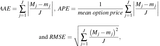
To measure the performance of suggested option prices model and Black-Scholes model are used average absolute error (AAE), average percentage error (APE), and root-mean error (RMSE). There are defined by Schoutens (2003) [21] as follows:

AAE =

J

∑

Mj−mj

J

, APE= 1

mean option price

J

∑

Mj−mj

J

andRMSE=

v u u t

_∑

j=1

(

Mj−mj

)2

J ,

whereMjare the market option price,bjare option price of the two-state Markov chain model with non-recombinant tree or Black-Scholes option price model for a different strike levels

j=1, . . .J.

All parameters of the model (u, vandy) and defined errors for the following companies ”American Express Company Common”(APX), ”Cisco Systems, Inc.”(CSCO), ”General Elec-tric Company Common”(GE), ”International Business Machines”(IBM), ”Intel Corporation”(INTC), ’JP Morgan Chase Co. Common S” (JPM), ”Coca-Cola Company (The) Common”(KO), ”3M Company Common Stock”(MMM), ”Merck Company, Inc. Common St”(MRK), ”Microsoft” (MSFT), ”Pfizer, Inc. Common Stock”(PFE), ”Procter Gamble Company”(PG), ”ATT In-c.”(T), ”The Travelers Companies, Inc. C”(TRV), ”Wal-Mart Stores, Inc. Common St”(WMT), ”Exxon Mobil Corporation Common”(XOM) are shown. The errors are determined by two-state Markov chain model with non-recombinant tree, Black-Scholes model and the market option price.

Results from errors show that, for the 30 stocks, two-state Markov chain model with non-recombinant tree gets closer option value to the market price of option than the price calculated by the Black-Schole model. The values of total summarized results are shown in Table 5.

6. Conclusion

The paper considers a discrete-time, two-state Markov chain market model with two traded securities: risky asset and risk-free asset. The uncertainty in the financial market is introduced as the daily changes of the risky asset are modulated by a discrete-time, two-state, Markov chain.

The issue of selecting risk-neutral measure in the Markov chain financial market model was also discussed. The method for valuation of a European style call option in our Markov chain market model is examined and presented.

Thus, by suitable specifications of parameters (u, v and y) the two-state Markov chain finan-cial market model can be constructed to reflect a possible feature of a real market, having bullish or bearish trends. It could create forgetful markets and markets with long memory, markets with different sorts of dependencies between assets returns. So, the two-state Markov chain market model has the bull and bear features of underlying asset price fluctuations, and it gives better results with the evaluation of option price of companies from DJIA.

Appendix

Here, it is presented in short the proposed method for finding all possible outcomes of a risky asset fornsteps. Withm0we define the outcome of the first step, which can be 1 or 0 meaning ”success” and ”failure”. Letm11, m10, m01 andm00denote the number of subsequences of the form ”success” - ”success”, ”success” - ”failure”, ”failure” - ”success” and ”failure” - ”failure”. Having totalnsteps we have the following:

m11+m10+m01+m00=n−1 (22)

Let first start with a procedure for determiningm11, m10, m01andm00. When the first step is ”success”m0=1 then the possible outcomes could be ”success” or ”failure” so we addwandv to each column in the matrix. When the first step is ”failure”m0=0 then the possible outcomes could be ”success” or ”failure” so we addyandxto each column in the matrix. In the next step if we have ”success” in the previous one which meansworywe add wandvto each column in the matrix. In case when we have in the previous step ”failure” which meansvorxwe addy

andxto each column in the matrix. The algorithm is given in Algorithm 1 box.

Algorithm 1 Calculate matrix of all possible states of risky asset using non-recombinant first order Markov chain

mat ←(uw;uv;dx;dy)

n←10

forn=3→ndo

[nCol,nRow] =size(mat)

for j=1→nCol do ifmat(j,:) =wthen

lastStepCol←[mat(j,:),w;mat(j,:),v]

else ifmat(j,:) =vthen

lastStepCol←[mat(j,:),x;mat(j,:),y]

else ifmat(j,:) =xthen

lastStepCol←[mat(j,:),w;mat(j,:),v]

else ifmat(j,:) =ythen

lastStepCol←[mat(j,:),x;mat(j,:),y]

end if end for

mat ←[mat,lastStepCol]

Using the those algorithms, we produce a list of all allowedmat a fixed depthn. Because we do not count the duplication of states, then a tree of depthnwill contain 2nstates.

Calculating the Markov tree is very difficult and needed high computational power but once we generated it we could use it many times to price many different options. For different options,S0, u, d, v, w, x,andywill be different, but the set of states will always be the same.

Conflict of Interests

The author declares that there is no conflict of interests.

Acknowledgments

The author was partially supported by the Bulgarian NSRF grant DTK 02/71, 2011.

REFERENCES

[1] H. Bhat, N. Kumar, Option pricing under a normal mixture distribution derived from the Markov tree model, Eur. J. Oper. Res. 3 (2012), 762-774.

[2] P. Carr, L. Cousot, Expensive mrtingales, Quantitative Finance, 3 (2005), 207-218.

[3] P. Carr, D. Madan, A Note on sufficient conditions for no arbitrage, Finance Res. Lett. 2(2005), 125-130. [4] P. Carr, L. Cousot, A PDE approach to jump-diffusions,Quantitative Finance, 1 (2011), 33-52.

[5] Charalambous C., Constantinide E. and Martzoukos S., Option Pricing on Non-Recombining Implied Trees Assuming Serial Dependence of Returns (2008), Available at SSRN: http://ssrn.com/abstract=1102215 or http://dx.doi.org/10.2139/ssrn.1102215

[6] L. Cousot, Conditions on option prices for absence of arbitrage and exact calibration, J. Banking Finance, 3 (2007), 3377 - 3397.

[7] J.C. Cox S.A. Ross, M. Rubinstein, Option Pricing: A Simplified Approach, J. Financial Economics (1979), 229 - 263.

[8] G. D’Amico J. Janssen, R. Manca, European and american options: The semi-markov case, Physica A, (2009).

[9] M. Davis, D. Hobson, The range of traded option prices, Math. Finance, 17 (2005), 1-14. [10] R. Elliot, L. Aggoun, J. Moore, Hidden Markov Models Springer-Verlag, (1995).

[11] R. Elliott, C.C. Liew, T.K. Siu, Characteristic functions and option valuation in a Markov chain market, Comput. Math. Appl. (2011), 65-74.

[13] L. Minkova, P. Radkov, Distributions related to a Markov chain and Application in Finance, Proceedings of the 11th Iranian Statistics Conference, August 28–30 (2012), Tehran Iran, 337 - 345.

[14] L. Minkova, E. Omey, new Markov binomial distribution, Commun. Statistics (2012), (to appear).

[15] N. Song, W.K. Ching, T.K. Siu, E.S. Fung, K. Michael, Option valuation under a multivariate markov chain model, 2012 5-th International Joint Conference on Computational Sciences and Optimization, 1 (2010), 177-181.

[16] R. Norberg, The markov chain market, ASTIN Bulletin - The Journal of the International Actuarial Associ-ation 33 (2003), 265-287.

[17] E. Omey, S.Van Gulck, Markovian black and scholes,Publications de l’institut math`ematique,79(93)(2006), 65 - 72.

[18] Omey E., J. Santos and S.Van Gulck, A Markov - binomial distribution, Applicable Analysis and Discrete Mathematics, 2 (2008), 38 - 50.

[19] S. Pliska, Introduction to mathematical Finance: Discrete time models, Blackwell Publishers, Malden, Mas-sachusetts (1997).

[20] Radkov P. and Minkova L., Markov - Binomial Option Pricing Model, in: Computing Data Analysis and Modeling: Complex Stochastic Data and Systems,(eds. Aivazian S., Filmoser P. and Kharin Yu.) Vol. 2, of Proceedings of the 9 - th Intern, Conf. Minsk, Publ. center of BSU (2010), Minsk, 169 - 172.

[21] W. Schoutens, S. Symens, The pricing of exotic options by Monte-Carlo simulations in a Levy market with stochastic volatility. International Journal for Theoretical and Applied Finance 6 (2003) 839C864.

[22] P. Tankov, R. Cont, Retrieving Levy processes from option prices: regularization of an ill-posed inverse problem, SIAM J. Control Optim. 1 (2006), 1-25.

[23] Valakevicius E.,Continuous Time Markov Chain Model of Asset Prices Distribution,Computational Science - ICCS 2009, 9-th International Conference, Baton Rouge, LA, USA, May 25-27, 2009, Proceedings, Part II, Lecture Notes in Computer Science, Springer, 5545 (2009), 598 - 605

10 20 30 40 50 60 70 0

5 10 15 20 25 30

strike level

option price

Two state Markov chain option price Market option price

Black Scholes option price

FIGURE 1. European call option on prices JPM under two state Markov chain model with non-recombinant tree tree, Black-Scholes model and market price. The current value S of the JPM is 42.81, the risk-free rateris 0.01% annually as a yield of 1-month Treasury bills. The dot line is a market option price for different strike prices. The dash line is a theoretical price by Black-Scholes model and the line is an option price under the Markov chain model with non recombinant-tree.

10 15 20 25 30 35 40 45 50

0 5 10 15

strike level

option price

Two state Markov chain option price Market option price

Black Scholes option price

TABLE1. Estimated equivalent martingale measure (EMM) parameters and respective error estimates (06 June 2014)

Company APX CSCO GE IBM

Expiry date 1m 3m 6m 34 days 3m 6m 1m 3m 6m 1m 3m 6m

S 92.80 24.70 26.77 185.98

σ 0.0121 0.0156 0.0112 0.0110

v 1.0155 0.9667 1.0551 1.0131 0.9706 0.9647 0.9801 1.0231 0.9475 0.9934 1.9691 1.0012 y 1.0013 0.9983 0.9953 0.9910 1.0010 1.0076 1.0000 1.0004 1.0002 0.9898 1.9998 1.0012 u 1.0122 1.0122 1.0122 1.0157 1.0157 1.0157 1.0112 1.0112 1.0112 1.0110 1.0110 1.0110

AAEmod 0.2408 0.3381 0.1602 0.3640 0.3126 0.2613 0.3176 0.2176 0.4218 0.3789 0.2263 0.1899

AAEBS 0.2660 0.5245 0.1851 0.8335 0.9724 1.6281 0.7623 0.3768 0.5047 1.1562 0.2989 0.3117

APEmod 0.0921 0.2259 0.1034 0.0457 0.0914 0.0447 0.0375 0.0263 0.0722 0.0526 0.0422 0.0381

APEBS 0.0992 0.2460 0.1062 0.6480 0.1278 0.2005 0.0807 0.0467 0.0928 0.0896 0.0596 0.0509

RMSEmod 1.332 2.2891 2.7645 0.2050 0.4205 0.0886 0.1105 0.1001 0.4164 0.8366 0.6320 1.0604

RMSEBS 1.382 2.3953 2.7960 0.2428 4641 0.2904 0.1865 0.1562 0.4556 1.0994 0.8264 1.2384

The risk-free rateris 0.25% annually. An appropriate Treasury bond is selected 1-month Treasury bill. Days to expiry of 1m option is 34 days, 3m - 70 days and 6m - 133 days

TABLE2. Estimated equivalent martingale measure (EMM) parameters and respective error estimates (06 June 2014)

Company INTC JPM KO MMM

Expiry date 1m 3m 6m 1m 3m 6m 1m 3m 6m 1m 3m 6m

S 27.66 56.63 40.89 143.71

σ 0.0126 0.0146 0.0301 0.0091

v 1.0266 0.9606 0.9717 1.0221 0.9783 0.9602 0.9992 1.0284 0.9580 1.0104 0.9583 0.9261 y 1.0001 1.0001 0.9860 1.0000 0.9999 1.0002 1.0000 1.0001 1.0004 1.0014 1.0003 1.0006 u 1.0128 1.0128 1.0128 1.0147 1.0147 1.0147 1.0306 1.0306 1.0306 1.0091 1.0091 1.0091

AAEmod 0.2799 0.4072 0.3253 1.0020 0.2029 0.5183 04776 0.2785 0.2790 0.3876 0.2176 0.2551

AAEBS 0.5696 0.7048 0.6408 3.2153 2.2775 0.6388 10.7481 15.9615 14.5118 0.6002 0.3864 0.2099

APEmod 0.1210 0.1656 0.0647 0.2094 0.0341 0.2144 0.0737 0.0721 0.0412 0.1007 0.0587 0.0599

APEBS 0.1523 0.1849 0.1865 0.3962 0.1809 0.3354 0.8795 0.5043 1.3920 0.1811 0.0664 0.0639

RMSEmod 0.5841 0.6736 0.1311 0.5224 0.1497 0.1805 0.1606 0.5606 0.1138 0.6704 1.2738 1.7679

RMSEBS 0.6084 0.6984 0.2432 0.8357 0.6262 0.3965 0.5679 1.8654 3.3806 0.9779 1.3713 2.0409

TABLE3. Estimated equivalent martingale measure (EMM) parameters and respective error estimates (06 June 2014)

Company MRK MSFT PFE PG

Expiry date 1m 3m 6m 1m 3m 6m 1m 3m 6m 1m 3m 6m

S 58.10 41.21 29.76 80.10

σ 0.0107 0.0142 0.0099 0.0091

v 1.0119 1.0246 0.9663 1.0129 0.9702 0.9678 1.0129 0.9766 0.9479 1.0012 1.0110 0.9871 y 0.9991 1.0034 0.9989 0.9994 1.0053 1.0058 1.0085 0.9999 1.0002 1.0012 1.0110 0.9777 u 1.0108 1.0108 1.0108 1.0143 1.0143 1.0143 1.0099 1.0099 1.0099 1.0092 1.0092 1.0092

AAEmod 0.2590 0.0997 0.3205 0.2861 0.1396 0.2677 0.5037 0.3554 0.4304 0.3644 1.0157 0.0386

AAEBS 0.4706 0.2523 0.1318 0.7210 1.1086 0.9247 0.5882 0.2798 0.2971 0.4326 1.0106 0.4903

APEmod 0.1224 0.1617 0.1020 0.0921 0.0711 0.1534 0.0429 0.0324 0.0563 0.0479 0.0286 0.0124

APEBS 0.1403 0.2341 0.0979 0.1183 0.0781 0.2711 0.0575 0.0314 0.0576 0.0539 0.1301 0.0755

RMSEmod 1.9735 0.5267 0.7407 0.7642 0.2399 0.4821 0.0517 0.0912 0.2422 0.5846 0.1226 0.0665

RMSEBS 2.0039 0.6378 0.7567 0.8265 0.3333 0.6811 0.0688 0.1039 0.2566 0.6186 0.3752 0.4173

The risk-free rateris 0.25% annually. An appropriate Treasury bond is selected 1-month Treasury bill. Days to expiry of 1m option is 34 days, 3m - 70 days and 6m - 133 days

TABLE4. Estimated equivalent martingale measure (EMM) parameters and respective error estimates (06 June 2014)

Company T TRV WMT XOM

Expiry date 1m 3m 6m 1m 3m 6m 1m 3m 6m 1m 3m 6m

S 35.10 97.97 77.32 100.55

σ 0.0096 0.0093 0.0084 0.0090

v 1.0000 0.9985 0.9983 0.9895 1.0623 0.9650 1.0000 1.0012 1.0110 1.0001 1.0110 1.0012 y 1.0427 0.9798 0.9769 0.9994 1.0002 0.9961 1.0102 1.0012 1.0110 1.0153 1.0110 1.0012 u 1.0096 1.0096 1.0096 1.0093 1.0093 1.0093 1.0090 1.0090 1.0090 1.0090 1.0090 1.0090

AAEmod 0.4471 0.2847 0.1316 0.1316 0.1384 0.2146 0.3445 0.1189 0.1488 0.2493 0.1283 0.3546

AAEBS 0.4429 0.3970 0.5355 0.5355 0.3525 0.3134 0.1945 0.3017 0.6584 0.3328 0.2564 0.2801

APEmod 0.0385 0.0659 0.0201 0.0201 0.0915 0.0252 0.0438 0.1040 0.0361 0.0366 0.0400 0.0586

APEBS 0.0452 0.0975 0.0421 0.0421 0.2015 0.0431 0.0732 0.1292 0.0545 0.0464 0.0584 0.0741

RMSEmod 0.1542 0.2435 0.2143 0.2143 0.7634 0.4156 0.2927 0.8015 0.5397 0.4937 0.1984 0.6504

RMSEBS 0.1863 0.2971 0.2778 0.4711 1.3304 0.6708 0.3762 0.8607 0.5951 0.5544 0.2799 0.8952

TABLE 5. Summarized error results

Type of errors 1m 3m 6m all AEEmoodvs.AEEbs 90.00% 86.87% 73.33% 83.4%

APEmoodvs.APEbs 100.00% 90.00% 86.87% 92.29%

RMSEmoodvs.RMSEbs 100.00% 93.33% 100.00% 97.77%

Total model error vs.Total BS error 96.66% 90.07% 86.73% 91.15%