Max Planck Institute for Demographic Research Konrad-Zuse Str. 1, D-18057 Rostock·GERMANY www.demographic-research.org
DEMOGRAPHIC RESEARCH
VOLUME 25, ARTICLE 1, PAGES 1-38
PUBLISHED 01 JULY 2011
http://www.demographic-research.org/Volumes/Vol25/1/ DOI: 10.4054/DemRes.2011.25.1
Research Article
The future of death in America
Gary King
Samir Soneji
c
°2011 Gary King & Samir Soneji.
2 Mortality and its patterns 3
3 Risk factors: Smoking and obesity 4
3.1 Relationship to mortality 5
3.2 Lag lengths 7
3.3 Measurement 8
3.4 Historical patterns 9
4 Forecasting methodology 11
4.1 Assessment of existing methods 11
4.2 Our approach 15
5 Mortality forecasts 15
6 Sources of uncertainty 19
7 Concluding remarks 22
8 Acknowledgements 23
References 24
A Appendix: Forecasting methodology 30
A.1 Overview of forecasting methodology 30
A.2 Bayesian hierarchical model 32
A.3 Search algorithm for setting priors 34
The future of death in America
Gary King1 Samir Soneji2
Abstract
Population mortality forecasts are widely used for allocating public health expenditures, setting research priorities, and evaluating the viability of public and private pensions, and health care financing systems. In part because existing methods forecast less accurately when based on more information, most forecasts are still based on simple linear extrapo-lations that ignore known biological risk factors and other prior information. We adapt a Bayesian hierarchical forecasting model capable of including more known health and de-mographic information than has previously been possible. This leads to the first age- and sex-specific forecasts of American mortality that simultaneously incorporate, in a formal statistical model, the effects of the recent rapid increase in obesity, the steady decline in tobacco consumption, and the well known patterns of smooth mortality age profiles and time trends. Formally including new information in forecasts can matter a great deal. For example, we estimate an increase in male life expectancy at birth from 76.2 years in 2010 to 79.9 years in 2030, which is 1.8 years greater than the U.S. Social Security Administra-tion projecAdministra-tion and 1.5 years more than U.S. Census projecAdministra-tion. For females, we estimate more modest gains in life expectancy at birth over the next twenty years from 80.5 years to 81.9 years, which is virtually identical to the Social Security Administration projection and 2.0 years less than U.S. Census projections. We show that these patterns are also likely to greatly affect the aging American population structure. We offer an easy-to-use approach so that researchers can include other sources of information and potentially improve on our forecasts too.
1Albert J. Weatherhead III University Professor, Harvard University, Institute for Quantitative Social Science,
1737 Cambridge Street, Cambridge MA 02138. E-mail: [email protected], http://GKing.Harvard.Edu.
2Assistant Professor, The Dartmouth Institute for Health Policy & Clinical Practice and The Norris Cotton
1. Introduction
Since 1950, U.S. life expectancy at birth has grown from68to78years. The U.S. also experienced considerable population aging resulting mainly from declining fertility and mortality. The elderly (≥ 65years) grew from14% of the population in1950to19% in2000, while the working age population (18 to 64 years) declined from60%to56%. These developments in population aging had massive implications for American life, as well as for the allocation of medical expenditures, public health efforts, research pri-orities, pension programs, Social Security, economic growth, and health care financing (Lee and Tuljapurkar 1997). Future American mortality patterns are of understandably widespread interest, despite their uncertainties. In this paper, we offer the first formal statistical forecasts of age and sex-specific U.S. mortality to include knowledge about commondemographic patternsin mortality, and large and well-studied biological risk factors.
The early demographic work of Graunt (1662), Huygens (Boyer 1947; Vollgraff 1950), Halley (1693) and Gompertz (1825) established two ubiquitous patterns that have con-tinued to hold up across many countries and time periods. First, age-specific mortality usually declines smoothly and gradually over time, with few sharp jumps from one year to the next. Second, time-specific mortality across age groups, known as “age profiles,” have a characteristic shape, with adjacent age groups having similar mortality rates. The vast majority of mortality forecasts to date have incorporated only the time-smoothness property; we make it possible to include as prior information (i.e., rather than either to ignore or require) both smoothness over time and age groups, when the data support it.
Smoking and obesity are two important risk factors, both with well-studied conse-quences for mortality and large changes over time. Smoking rates steadily declined over the last half century, and obesity rates have rapidly increased in the last thirty years. Most American mortality forecasts ignore these patterns and are based only on simple extrapo-lations without covariates, and so include these risk factors only indirectly. Other methods study these risk factors directly but do not include the known tendency of demographic patterns to be smooth over time and age. We directly measure and include both risk factor and known demographic patterns in the same forecasting model, which allows forecasts to take note of these factors if — and only if — the data support their inclusion.
uncertainty (which we also measure and report) but fortunately structural breaks tend to be rare.
We forecast mortality by single year of age and sex for the next twenty-five years in the U.S. We also offer guidance about the use of our approach that will enable other scholars to produce even better forecasts than ours when new covariates or other infor-mation become available. Methods such as ours tend to be the most accurate available when the underlying data generating process is uncertain because empirical regularities. These methods should not be confused with models optimized for making causal infer-ences, which is a different task and requires other approaches (e.g., Ho et al. 2007; Robins 2008). Indeed, none of our results should be seen as claims about the causal effects of obesity, smoking, or any other factor.3
First, we summarize known demographic and risk factor information useful for fore-casting in Sections 2 and 3. Second, we assess existing forefore-casting methods in Section 4.1 and our approach in Section 4.2. Third, we present our mortality forecasts in Section 5. Fourth, we discuss sources of uncertainty and possible difficulties with our approach in Section 6. Finally, we present mathematical details of our forecasting method in the appendices.
2. Mortality and its patterns
We first discuss an important issue in measuring mortality and then illustrate the venerable pattern of how mortality smoothly changes over time and age. We use patterns such as these as prior information to improve the forecasts when supported by the data.
MeasurementThe most commonly used indicator of mortality in demography is the mortality rate(usually writtennxmxfor age group[x, x+nx)). The mortality rate is the
number of deaths in a time period and age group divided by the person-years of exposure to the risk of death. In practice, the exposure time is not known and so must be estimated based on assumptions about when deaths occur during each time interval. This is not a major issue for most demographic analyses, but it is a serious issue for forecasting. Exposure in the in-sample data (used to construct the forecast) and exposure in the the out-of-sample data (used to validate the forecast) both must be estimated. As such, validating a forecast based onnxmxis usually impossible, since assumptions about future exposure
can always be adjusted to apparently improve the forecasts.
3Different research goals typically require entirely different specifications: For example, in estimating the
Our solution to this problem is to use theconditional probability of deathas our mea-sure. This quantity is usually written asnxqxfor age group[x, x+nx). The conditional
probability of death is the number of deaths in a time period and age group divided by the population alive at the start of that time period, and so is easy to interpret. Since both components are directly observable,nxqxis also directly observable. As such, forecasts
that withhold known mortality so it can be used for validation are vulnerable to being proven incorrect, which is required for scientific progress.
Empirical regularitiesBetween1950and2007, U.S. age-specific mortality was lo-cally smooth and maintained an age profile similar to the pattern shown in the left panel of Figure 1. We measurenxqxby each single year of age from0 to100(with 100 as
the start of an open age interval and∞q100= 1) between1980and2007. We follow the common demographic convention of dropping the left subscript when the age group is a single year of age.4Smoothness within a given year can be seen by the small incremental changes in log-mortality across age groups. The consistent pattern starts with high infant mortality followed by a rapid decline until approximately age10. Mortality then increases to a local maximum, the so-called accident hump especially prominent in males. Adult log-mortality then increases nearly linearly until an apparent deceleration starting at about age90.
Time trends of mortality are also locally smooth and decline over time (Figure 1, right panel) consistent with patterns in most other time periods in advanced industrialized countries (Gompertz 1825; Keyfitz 1982; McNown 1992). Smoothness for a given age can be seen by small incremental changes in log-mortality over time. The pace of the decline differs slightly among ages and over some short time intervals. For example, age 0 mortality decreased fastest during the 1990s and slowed in the 2000s. The pace of mortality decline over time was quite similar among adults aged 60-80 years. A similar pace of decline among the oldest-old ages (≥85 years) observed in the U.S. has been well documented with high-quality demographic data in over two dozen other countries (Kannisto et al. 1994).
3. Risk factors: Smoking and obesity
In this section, we discuss evidence of tobacco consumption and obesity’s effect on mor-tality. Covariates need not have a causal relationship to mortality to ensure predictive success, but the causal literature is certainly helpful in making choices.
4To determine death counts, we use the Mortality Detail Files 1980–2007, containing information on all deaths
Figure 1: Observed U.S. male mortality, age and time domains
0 20 40 60 80 100
−8 −6 −4 −2
1950
2007
1950 1960 1970 1980 1990 2000 −8
−6 −4 −2
0
10
20
30 40 50
60 70
80 90
Ages
Age Year
log (q
x
)
Notes: The left panel shows the age profile of male log-mortality (measured by the conditional probability of death) in 1950 and 2007. The right panel shows male log-mortality for select ages observed between 1950 and
2007. Ages are listed along the left side (e.g., “60” represents age[60,61)years).
3.1 Relationship to mortality
The strong link between cigarette smoking and increased risk of mortality has been well established since1950(Doll 1999; Parascandola 2004). Cigarette smoking increases the risk of cardiovascular disease, lung cancer, chronic obstructive pulmonary disease mor-tality, and nearly fifty other causes of death. After adjusting for several known mortality risk factors, Jacobs et al. (1999) found smokers’ hazard of death1.3times greater than non-smokers and the attributable risk of smoking to be23%. In the fifty-year followup of their seminal study, Doll et al. (2004) estimated male cigarette smokers died ten years younger than nonsmokers, on average.
inflam-matory responses. The result is a cycle of further metabolic dysfunction and inflaminflam-matory responses that contribute to cellular stress. For example, excessive oxidation of glucose or free fatty acids by mitochondria creates oxidative stress, which can damage cellular structures.
Within the scientific community, there is uncertainty on obesity’s effect on mortality at the population level (Crimmins, Preston, and Cohen 2011). There is general consensus of excess age-specific mortality among the class I, II, and III obese (Fontaine et al. 2003; Olshansky et al. 2005; Stewart, Cutler, and Rosen 2009).5 Yet, how much the overweight experience leads to excess age-specific mortality remains an open empirical question. In their careful prospective analysis of 900,000 adults, Prospective Studies Collaboration (2009) considered the relationship between obesity and mortality among current cigarette smokers and those who never smoked regularly. Among smokers, compared to the normal weight group, the risk of mortality was higher for the underweight, approximately equal for the overweight, higher again for class I obese, and higher still for class II obese. Among non-smokers, compared to the normal weight group, the risk of mortality was no higher for the underweight or overweight groups, was higher for the class I obese, and higher still for the class II obese.
Equally uncertain is the extent to which obesity affects life expectancy. Peeters et al. (2003) found an estimated reduction in life expectancy at age forty of six years for obese males and seven years for obese females, compared to their non-obese counter-parts. Fontaine et al. (2003) found an estimated decline in male life expectancy at age 50 ranging from one to seven years for those ranging from BMI 30 to 45+, respectively. A similar decline was noted in female life expectancy. Recently, Preston and Stokes (2010) found an estimated gain in life expectancy at age fifty from hypothetically redistributing the obese into optimal BMI categories between 0.6 and 1.9 years for males and 0.8 to 1.6 years for females.
Flegal et al. (2010) suggest the mortality risk associated with obesity may be changing over time. More effective medical management of obesity related complications using existing therapeutic agents may mitigate the impact on mortality and longevity for some. Emerging biological knowledge of the mechanisms and signaling pathways by which genetic and environmental factors interact to favor weight gain and disrupt metabolism is also opening the possibility of new therapeutic intervention (Baur et al. 2006). Although compliance with medical recommendations in a population that also experiences difficulty complying with dietary advice may not be very high.
A population’s health is a complex multi-dimensional concept that changes over age, time, and across countries. We consider cigarette smoking and obesity, though there
cer-5 The World Health Organization classification of BMI: underweight (BMI≤18.5), normal weight
tainly are other important risk factors. The interaction of risk factors is quite likely, as well. Freedman et al. (2006) found the mortality risk among obese smokers, even young obese smokers, far exceeded the sum of their individual risks. Considerable variation in mortality risk may also exist among individuals, even within a specific sub-population. For example, Wessel et al. (2004) note substantial differences in cardiorespiratory fitness among females at all levels of obesity, but the precise and complex interactions among physical fitness, obesity, and mortality remain largely unknown (Allison et al. 2003). In-cluding all necessary interactions and sub-population effects to build a completely spec-ified causal model would be an important task, but is not the subject of this paper. Our alternative strategy of forecasting based on causally informed empirical regularities is likely to be somewhat safer, at least until considerably more data become available.
3.2 Lag lengths
Contemporaneous relationships and lagged relationships with mortality are two approaches to using covariates in forecasting. Using the contemporaneous relationship between co-variates and mortality is generally not a good idea for two reasons. First, we would not expect the risk factors to instantly affect mortality. Second, using the risk factors at time
tto predict mortality at timetrequires one to separately forecast covariates prior to fore-casting mortality, since knowledge of the covariates would be required at timet+kfor ak
step ahead forecast. This extra forecasting step is not only inconvenient and model depen-dent, but it also propagates considerable additional uncertainty into the ultimate mortality forecasts.
In contrast, using lagged covariates in mortality forecasting models is typically a more objective, less model-dependent, and less uncertain approach. We thus lag the covariates in a cohort-based analysis. That is, we lag the risk factorskyears in time while keeping the cohort, which iskyears younger, the same. We then use a one-step ahead forecasting procedure with the final observed year of covariate values to forecast k years into the future. This approach bases forecasts on risks already experienced by the population rather than on risks predicted to occur in the future.
(2007) recently found a strong association between childhood obesity and coronary heart disease mortality between ages 25 and 60.
Thus, we keep the lag lengthkto approximately what we learn from the life course perspective, which is aboutk= 25years, for both smoking and obesity, although the lag value need only be approximate given the high autocorrelation in mortality. We demon-strate this point by also considering shorter lags,k = 5,10,15, and20years in Section 6. When lagging far enough back so that the covariate would not be meaningful, such as smoking rates for infants, we drop the covariate. A crucial advantage of our statistical methodology is that it enables us to use different covariates for forecasting different age groups while still borrowing strength in estimating all the cross-sections together, and smoothing over age and time appropriately.
As Soneji and King (2011) note, period effects may also strongly affect mortality, in addition to cohort effects. For example, the 1964 U.S. Surgeon General’s Report on Smoking and Health (Office of the Surgeon General 1964) marked a period of intense anti-tobacco public health campaigns. The collection, now totaling over thirty reports, fo-cused on changing behavior, attitudes, and knowledge among potential and current smok-ers. Unlike a cohort-specific model, which incorporates time-lagged correlation between potential covariates and mortality, a period-specific model would require the prediction of covariates for ages in the future. Also noteworthy is the current debate within the demographic research community on whether period life expectancy is biased because of changes in the timing or age of mortality (Bongaarts and Feeney 2003; Guillot 2003; Wilmoth 2005). Such changes in the timing of death may result, for example, from the considerable decline in U.S. smoking.
3.3 Measurement
We estimate historical smoking prevalence from 1955 to 2007 from national-level cross-sectional surveys, including the 1955 Current Population Survey and seventeen National Health Interview Surveys (NHIS) beginning in 1966. From 1955 to 1991, a respondent was considered a current smoker if he or she responded affirmatively to the questions “Have you smoked at least 100 cigarettes in your entire life?” and “Do you now smoke?”. In 1992, the second question changed to “Do you now smoke every day, some days, or not at all?”. Since 1992, a current smoker was defined as someone who has smoked at least 100 cigarettes in their life and currently smokes every day or some days. In all our analyses, survey weights calculated by the National Center for Health Statistics are incorporated so that respondents represent their population share. Non-response through refusal to answer, lack of knowledge, or inability to ascertain tobacco usage was less than 1.4% for all years of the survey.
including the 1959–1962, 1971–1975, and 1976–1980 waves of the National Health and Nutrition Examination Survey and annual NHIS since 1981. A respondent is considered obese if his or her Body Mass Index (BMI) is30kilograms per meter squared or greater. We recognize the possible disadvantage combining information from surveys with differ-ent methodologies and a single BMI threshold for obesity (Mehta and Chang 2009). BMI itself may also have limitations as a measure of apidosity because it does not differentiate between fat mass (e.g., visceral fat) and fat-free lean mass (Bergman et al. 2006; Snijder et al. 2006). Several studies argue that a greater percentage of fat mass increases mortality risk, especially among the elderly. A greater percentage of fat-free lean mass, however, may decrease mortality risk (Heitmann et al. 2000). Yet in their systematic review of54 cohort studies, Romero-Corral et al. (2006) note the higher BMI, the better the discrimi-natory power for body fat and lean mass. However, the signal from the pattern of obesity change in the U.S. appears to overwhelm any such measurement noise. Other thresholds for obesity, and other measures such as average BMI, do change the forecasts, but do not have a major impact on the results. The resulting data is a rich history of the best existing height and weight measurements over the last 47 years.
Finally, following Murray and Lopez (1996) and others, we use a linear time trend as a proxy for technological progress. This is a crude measure, but we have not found dra-matic differences with other basis functions so long as our priors for demographic patterns are also included. Our preliminary experiments using patents and National Institutes of Health research funding also does not seem to have a large effect, although this is worth much further study.
3.4 Historical patterns
We estimate smoking and obesity prevalence for males and females ages 0 to 100 between 1955 to 2007. As with mortality, we expect the prevalence of these risk factors to change smoothly over time, though the observed values are more noisy because they are based on random samples. We therefore apply the smoothing techniques described in Section 4.2 which also enable us to interpolate prevalence during years without sample data.
Figure 2: Smoking and obesity prevalence over time
1960 1970 1980 1990 2000 0.0 0.1 0.2 0.3 0.4 0.5 0.6 Age 20 40 60 80
1960 1970 1980 1990 2000 0.0 0.1 0.2 0.3 0.4 0.5 0.6 Age 20 40 60 80
1960 1970 1980 1990 2000 0.00 0.05 0.10 0.15 0.20 0.25 0.30 0.35 Age 20 40 60 80
1960 1970 1980 1990 2000 0.00 0.05 0.10 0.15 0.20 0.25 0.30 0.35 Age 20 40 60 80 Year Year Pre v alence Pre v alence
Smoking, Female Smoking, Male
Obesity, Female Obesity, Male
Notes: Smoking (top graphs) and obesity (bottom graphs) for females (on the left) and males (on the right) for selected ages (in colors). Observed data are shown as open circles and smoothed estimates as lines. Ages
Both sexes experienced a dramatic increase in obesity, as measured by excess BMI, with the sharpest increases occurring among the young (Figure 2, lower panels). For example, the prevalence of obesity increased from 10% in 1961 to 28% in 2007 among forty-year old males. Similarly aged females experienced an increase from 13% in 1961 to 27% in 2007. The fastest increase has occurred since 1990 for all age groups and both sexes.
The relationship between obesity, morbidity, and mortality may change over time with advancements in medicine. Pharmacological innovations may have contributed to reductions in cardiovascular disease (CVD) risk factors over time, an important medical complication of obesity. Gregg et al. (2005) observed secular reductions in hypertension and high total cholesterol level among all BMI groups. A crucial exception is diabetes mellitus; this CVD risk factor nearly tripled among the obese from 1960 to 2000. Our linear trend will proxy for some of this and other technological progress.
4. Forecasting methodology
We discuss here issues with existing methods and then introduce our approach, which attempts to build on the existing methods and address some of the issues they raise.
4.1 Assessment of existing methods
Ideally, a mortality forecast would simultaneously incorporate the effect of the rapid in-crease in obesity and the steady decline in cigarette consumption, while still maintaining the long-standing patterns of smooth mortality age profiles and time trends. At the same time, these patterns only affect the forecasts if not greatly contradicted by the in-sample data. Forecasting methods to date have not been able to incorporate this combination of properties. First, by construction, purely extrapolative methods cannot include informa-tion about the direct effects of risk factors with known health effects. Second, because of various independence assumptions, existing methods that allow for the incorporation of key risk factors often yield forecasts that violate the well known demographic patterns of smooth age and time profiles.
We illustrate these problems by using the two most common existing forecasting methods: the time-series based Lee-Carter approach (Lee and Carter 1992) and least squares (LS) regression. We use 1980–2007 U.S. male mortality data to forecast through the year 2030.
Sec-ond, we consider a forecast of log-mortality as a linear function of time (Figure 3, second column). We write this model as:
E(log(qa,t)) =β(0)a +βa(year)yeart. (1)
This forecast yields nearly identical results to those of Lee-Carter. Third, we consider a forecast of log-mortality as a linear function of time and smoking lagged by 25 years (Figure 3, third column). We write this model as:
E(log(qa,t)) =
(
βa(0)+βa(year)yeart, ifa <50
βa(0)+βa(year)yeart+βa(smoking)smokinga−25,t−25, ifa≥50
(2)
where smokinga−25,t−25is smoking prevalence 25 years earlier in age and 25 years earlier in time. The results here are plausible for some ages and implausible for others; the age profiles grow increasingly non-smooth. For example, mortality is low for 30-year-olds, enormously higher for 35-year-olds and almost nonexistent for 40-year-olds. This fore-cast is very far from any historical experience and so cannot be taken seriously. Fourth, we consider a forecast of log-mortality as a linear function of time, smoking lagged by 25 years, and obesity lagged by 25 years (Figure 3, fourth column). We write this model as:
E(log(qa,t)) =
βa(0)+β(year)a yeart, ifa <50
βa(0)+β(year)a yeart+β
(smoking)
a smokinga−25,t−25
+βa(obesity)obesitya−25,t−25, ifa≥50
(3)
where smokinga−25,t−25is similarly defined and obesitya−25,t−25is obesity prevalence 25 years earlier in age and 25 years earlier in time. The dubious time series plot and highly non-smooth age profile plot are implausible, with no historical experience to support such a pattern.
Figure 3: Male all-cause log-mortality forecast: Lee-Carter, linear time trend, time+smoking, and time+smoking+obesity
1990 2010 2030 −10 −8 −6 −4 −2 Year 5 10 15 20 25 30 35 40 45 50 55 60 65 70 75 80 85 90 95 Age
1990 2010 2030 −10 −8 −6 −4 −2 Year 5 10 15 20 25 30 35 40 45 50 55 60 65 70 75 80 85 90 95
1990 2010 2030 −10 −8 −6 −4 −2 Year 5 10 15 20 25 30 35 40 45 50 55 60 65 70 75 80 85 90 95
1990 2010 2030 −10 −8 −6 −4 −2 Year 5 10 15 20 25 30 35 40 45 50 55 60 65 70 75 80 85 90 95
0 20 40 60 80 100 −10 −8 −6 −4 −2 Age 1990 2000 2010 2020 2030
0 20 40 60 80 100 −10 −8 −6 −4 −2 Age
0 20 40 60 80 100 −10 −8 −6 −4 −2 Age
0 20 40 60 80 100 −10 −8 −6 −4 −2 Age log (q x ) log (qx )
Lee−Carter Linear Model: Time
Linear Model: Time+Smoking
Linear Model: Time+Smoking+Obesity
Notes: Log-mortality forecasts by the Lee-Carter approach (1st column) and three least squares regressions: time (2nd column), time and smoking lagged 25 years (3rd column), and time, smoking lagged 25 years, and obesity lagged 25 years (4th column). Observed mortality are shown as open circles. Ages are listed along
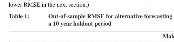
ValidationWe now show that the existing forecasting methods studied above, which produce implausible results based on historical experience, also turn out to be suboptimal when evaluated in rigorous out-of-sample tests. To illustrate these tests, we set aside the last ten years of observed historical mortality (1998-2007) as the validation period and create forecasts based only on the earlier data (1980-1997). We then calculate the average root mean square error (RMSE) of the out-of-sample data for all ages and all years in the validation period, for both male and female mortality. We repeat the same RMSE calculation for each of the four methods illustrated in Figure 3.
The results appear in the first four rows of Table 1. Out-of-sample RMSE is lowest for the models that ignore the most information — the Lee-Carter models and least squares with only time as a covariate, for both males and females. (We discuss our method and its lower RMSE in the next section.)
Table 1: Out-of-sample RMSE for alternative forecasting methods, based on a 10 year holdout period
Male Female
Lee-Carter 0.0140 0.0041
Least Squares Regression: Time 0.0135 0.0044 Least Squares Regression: Time+Smoking 0.0184 0.0065 Least Squares Regression: Time+Smoking+Obesity 0.0310 0.1606
Our Mortality Forecast 0.0079 0.0039
4.2 Our approach
We employ a Bayesian hierarchical modeling approach developed by Girosi and King (2008) to incorporate both the key risk factors of smoking and obesity and the long-standing demographic patterns of smooth mortality age profiles and time trends into the same forecasting approach (King and Soneji 2011). In this approach, risk factors and time are included in linear regression models as measured covariates. Demographic informa-tion on smoothness of expected mortality across age groups and time periods enters the model as Bayesian priors. The priors are not merely on difficult-to-interpret coefficients, as in classic Bayesian approaches, but instead are stated as beliefs about aspects of ex-pected mortality such as smoothness across age groups and time periods, which is what prior demographic research has taught us. The method also estimates the set of regres-sions from age-specific forecasts together, rather than making implausible independence assumptions across age groups or time periods, or requiring the same covariates for all cross-sections (such as requiring tobacco consumption among infants).
The Bayesian priors thus incorporate previous empirical patterns and formalize quali-tative knowledge demographers have gained over the last 350 years. The Bayesian model uses demographic and risk factor information, but is designed to down-weight or ignore it if contradicted by observed empirical patterns. The priors only have their effect on forecasts in areas where the data are weak, and the risk factors only have an effect on the forecasts if the hypothesized pattern is found in the in-sample data. We summarize the details of the statistical methods we use, along with a worked example, in the Appendix.
Girosi and King (2008, Chapters 11–13) present extensive tests of the model for nu-merous mortality data sets in many countries. They show that including information in this model in the way we do substantially improves out-of-sample forecasts. Thus, to these validation results, we add the final row of Table 1; this reports the out-of-sample RMSE for our forecasts, which are lower than the other for methods reported, consistent with the results of Girosi and King (2008).
5. Mortality forecasts
E(log(qa,t)) =
βa(0)+β(year)a yeart, ifa <50
βa(0)+β(year)a yeart+β
(smoking)
a smokinga−25,t−25
+βa(obesity)obesitya−25,t−25, ifa≥50
(4)
where smokinga−25,t−25 is smoking prevalence and obesitya−25,t−25 is obesity preva-lence 25 years earlier in age and 25 years earlier in time. The regression coefficients,
β, are drawn from a Bayesian posterior distribution, as described in Section A2. The covariates are not projected or forecasted into the future. Rather we base forecasts on past risks already experienced by the population. We discuss forecasts of mortality, life expectancy, and the population age structure. We also compare our forecasts with official U.S. projections.
Future mortalityIn Figure 4, we present our mortality forecasts in the time and age domains and highlight key properties and differences between the sexes and among age groups. Unlike the demographically unreasonable least squares forecasts with the method given in Figure 3, our forecasts maintain common historical demographic patterns: they are smooth over time, as seen in the solid lines in the upper panels of the figure, and smooth across age groups, as shown in the bottom panels (color-coded by year).
Figure 4: Male and female log-mortality over time and age groups for our model including time, smoking, obesity, and smoothness priors
1980 1990 2000 2010 2020 2030
−8 −6 −4 −2 0 Age 10− 14 15− 19 30− 34 35− 39 40− 44 45− 49 50− 54 55− 59 60− 64 65− 69 70− 74 75− 79 80− 84 85− 89 90− 94
1980 1990 2000 2010 2020 2030
−8 −6 −4 −2 0 Age 10− 14 15− 19 30− 34 35− 39 40− 44 45− 49 50− 54 55− 59 60− 64 65− 69 70− 74 75− 79 80− 84 85− 89 90− 94
0 20 40 60 80 100
−8 −6 −4 −2 0 1990 2000 2010 2020 2030
0 20 40 60 80 100
−8 −6 −4 −2 0 1990 2000 2010 2020 2030 log (q x ) log (qx ) Male Female
Notes: The top panel shows observed male (left) and female (right) log-conditional probability of death (in circles) along with model forecasts (solid lines) for selected ages. The bottom panels give the age profile of model forecasts between 1980 and 2030, again for males (left) and females (right), and color-coded for select
years. SSA forecasts are represented by+signs. Age groups are listed along the left side of each upper
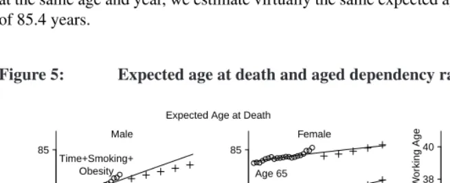
Life expectancyPeriod life expectancy is the expected remaining life of an individual of a given age who experiences the age-specific mortality of a given year (Preston, Heuve-line, and Guillot 2001). In the left and center panels of Figure 5 for males (left) and females (center), we present this statistic for ages 0 and 65, calculated from our forecast conditional probabilities of death6. For males, our estimates (given by solid lines) are substantially higher than SSA’s projections (given by +). For males, we estimate life ex-pectancy at birth to increase steadily from 75.6 years in 2007 to 79.9 years in 2030. In comparison, the SSA forecast in 2030 is 78.1 years. For females, we estimate virtually the same life expectancy at birth in 2030 as the SSA of 81.9 years.
We also calculate the expected age at death among those alive at age 65 (equal to the sum of 65 years and life expectancy at age 65 in a period life table) as shown in the upper lines of the left and center panels of Figure 5. For males age 65 in 2030, we estimate the expected age at death to be 84.4 years, compared to 83.4 years by the SSA. For females at the same age and year, we estimate virtually the same expected age at death as the SSA of 85.4 years.
Figure 5: Expected age at death and aged dependency ratio over time
1990 2010 2030 75
80 85
Age 0 Age 65
SSA Time+Smoking+
Obesity
1990 2010 2030 75
80 85
Age 0 Age 65
1990 2010 2030 32
34 36 38 40
Ratio of Elder
ly per 100 W
or
king Age
Year Year Year
Expected Age at Death
Male Female
Aged Dependency Ratio
Notes: The left and middle panels give expected age at death for males (left) and females (middle) at age 0 and
65 under the time+smoking+obesity model, as well as Social Security Administration projections (+). (In
a period life table, the expected age of death equals the sum of life expectancy and age.) The right panel
gives the ratio of elderly (≥65years) to the working age population (between 20 and 64 years).
6To close the life table, we follow the approach of Horiuchi and Coale (1982) and Preston, Heuveline, and
Aging population structureWe calculate the ratio of the number of elderly≥65years to the number of adults between ages 20 to 64 years, which is known as theaged dependency ratio. For programs relying on intergenerational transfers of wealth like Social Security, larger ratios imply greater strain on the working age population to support the elderly dependent population. The right panel of Figure 5 gives the aged dependency ratio from 1980 to 2030. In 1980, there were 30.5 elderly per 100 people of working age. We estimate that the ratio rises steadily over time and faster than officially projected. By 2030, we forecast 40.6 elderly will be alive per 100 people of working age. In contrast, the SSA projects the ratio lower, 39.5 per 100 people of working age. The difference of 1.1 additional elderly per 100 people of working age is considerable when compared to historical data in the U.S. and elsewhere.
6. Sources of uncertainty
Physicians, policy makers, and public health officials make many decisions based on mor-tality forecasts, regardless of the uncertainties. Nevertheless, any user of these or other forecasts should be aware of how forecasts can go wrong. We may have reduced the uncertainties considerably by including more demographic and risk factor information in the forecasts, but the following unknowns remain.
First, surveys used to estimate obesity and smoking prevalence have sampling error, partially mitigated by smoothing over time and large sample sizes (11,000–116,000); they also have self-reporting error. Second, death and population counts may also be measured with error, especially for individuals without birth certificates such as elderly southern blacks. Third, growing social stigmas of smoking and obesity may lead to under-reporting of smoking behavior and weight (Ezzati et al. 2008). However, error in self-reports would not likely cause many to under-report their weight so much as to become recategorized as overweight instead of obese, and in any event will only bias our analyses to the extent that the stigma itself varies substantially over time, regardless of the degree to which the prevalence of smoking and obesity change.
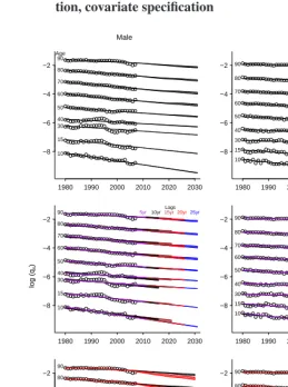
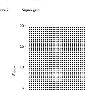
We first study uncertainty due the choice of Bayesian priors used to represent the knowledge that expected mortality is smooth over time and over age groups. We study this prior uncertainty with a version of “robust Bayesian analysis” by using a class of priors instead of only one, and with the result producing a range of forecasts instead of a single point estimate (e.g., Berger 1994; King and Zeng 2001). Thus, for each covariate specification, we use all prior specifications that pass through our search algorithm for setting priors described in Appendix A3. The result of this process is a large number of forecasts that we present as an uncertainty interval in the top panels of Figure 6. Prior uncertainty does affect the forecast, but the pattern in the forecasts remains unambiguous. In the middle panels of Figure 6, we show the male and female forecasts time, smok-ing, and obesity, and with varying lag length specifications. Lag lengths are color coded and labeled in five-year intervals from 5 years at the left to 25 years at the right. Prior-based model dependence is also represented in this figure by plotting the whole forecast interval for each given lag length. The results indicate a lack of strong dependence on the lag length. Recall that, with our cohort approach, including ak-year lag of the covariates, produces a forecastkyears into the future. This is why, for example, the purple-colored 5-year forecasts extends until 2012, whereas the black-colored 10-year forecasts go until 2017. Thus, to compare these two forecasts directly, we must project the 5-year forecasts an extra five years or examine where the 10-year lag forecast projects when it is only 5 years out. In most cases, eachk-year forecast is consistent with the(k+ 5)-year forecast; slight exceptions are approximately within the prior uncertainty bounds, represented by multiple lines for each lag length.
The bottom panels in the figure portray model dependence due to the choice of co-variates, with the prior uncertainty interval included as before. The red-colored forecast intervals include only time and lagged smoking, whereas the black-colored intervals in-clude time, lagged smoking, and lagged obesity. Although this is not a causal model, it does make some sense that most of the forecast intervals that include obesity lead to higher mortality forecasts after age 50.
Figure 6: Model-based uncertainty: Prior specification, lag length specifica-tion, covariate specification
1980 1990 2000 2010 2020 2030 −8 −6 −4 −2 Age 15 10 30 40 50 60 70 80 90
1980 1990 2000 2010 2020 2030 −8 −6 −4 −2 15 10 30 40 50 60 70 80 90
1980 1990 2000 2010 2020 2030 −8
−6 −4 −2
Lags 5yr10yr15yr20yr25yr
15 10 30 40 50 60 70 80 90
1980 1990 2000 2010 2020 2030 −8
−6 −4 −2
Lags 5yr10yr15yr20yr25yr
15 10 30 40 50 60 70 80 90
1980 1990 2000 2010 2020 2030 −8 −6 −4 −2 Time+Smoking+Obesity Time+Smoking 15 10 30 40 50 60 70 80 90
1980 1990 2000 2010 2020 2030 −8 −6 −4 −2 15 10 30 40 50 60 70 80 90 log (q x ) Year Year Male Female
Notes: For males (in the left column) and females (in the right column), the first row shows forecast uncertainty intervals due to changes in the prior specification, the second row due to different lag lengths, and the third row due to covariate specification (time+smoking or time+smoking+obesity, each with plausible prior specifications lagged 25 years). Observed log-conditional probabilities of mortality are shown as open
7. Concluding remarks
By including more health and demographic information than has been previously possi-ble, we draw several important conclusions about future mortality patterns. First, by in-corporating information on the steady decline in cigarette smoking prevalence and rapid increase in obesity, we forecast mortality may decline faster than officially projected, es-pecially for males≥ 50years. Second, the pace of mortality decline may be faster for males than for females. Third, the impact on the demography of future populations is profound. We find faster gains in life expectancy and faster aging of the U.S. population than officially projected.
The age profiles and time trends of our mortality forecasts are smooth and maintain the same venerable demographic patterns of historical mortality in the U.S. and most other countries and time periods. By incorporating risk factors with known health effects (smoking and obesity) we are able to produce more informed mortality forecasts in a statistically sound manner.
Our findings, along with those of Olshansky (1988); Lee and Carter (1992); Lee and Miller (2001); Oeppen and Vaupel (2002); Olshansky et al. (2005); Li and Lee (2005); Wang and Preston (2009); Stewart, Cutler, and Rosen (2009); Olshansky et al. (2009) em-phasize the importance of continual development and assessment of forecasting methods and the potential utility of including risk factors in forecasts. The careful inclusion of risk factors, while maintaining ubiquitous demographic properties, will allow demographers to improve the quality, accuracy, and transparency of mortality forecasts.
We must keep in mind that these forecasts are at the population level, based on time-lagged correlations, and do not necessarily imply causality at the individual level. Addi-tional relevant covariates may further inform future forecasts, such as trends in marriage, education, and immigration. Although traditional omitted variable or confounding bias are not relevant here, as they are in estimating causal effects, one may be able to improve our forecasts with such additional information.
Future US mortality patterns may be, at least in part, affected by future mortality pat-terns elsewhere. As Torri and Vaupel (2011) note, this cross-national association may occur through several pathways including the transfer of scientific knowledge and in-novations (e.g., pharmaceuticals, standards of care), introduction of pathogens through migration and travel, and macro-level political, social, and economic forces. Our method-ology and framework may prove useful for future global forecasts of mortality that take into account relevant contextual factors and incorporates demographic commonalities and differences.
Adminis-tration (Sloan et al. 2004) and Medicare (Wright 1986). Whether obesity-related mortal-ity represents net financial gains or losses to Social Securmortal-ity and Medicare remain open questions. Much depends on the morbidity associated with obesity, early work disability, earnings, and mortality before and after retirement age.
8. Acknowledgements
References
Allison, D.B., Wang, C., Redden, D.T., Westfall, A.O., and Fontaine, K.R. (2003).
Obe-sity and years of life lost−reply.Journal of the American Medical Association289(14):
1777–1778.doi:10.1001/jama.289.14.1777-c.
Baker, J., Olsen, L., and Sørensen, T. (2007). Childhood body-mass index and the risk of
coronary heart disease in adulthood. The New England Journal of Medicine357(23):
2329–2337.doi:10.1056/NEJMoa072515.
Baur, J., Pearson, K., Price, N., Jamieson, H., Lerin, C., Kalra, A., Prabhu, V., Allard, J., Lopez-Lluch, G., Lewis, K., Pistell, P., Poosala, S., Becker, K., Boss, O., Gwinn, D., Wang, M., Ramaswamy, S., Fishbein, K., Spencer, R., Lakatta, E., Le Couteur, D., Shaw, R., Navas, P., Puigserver, P., Ingram, D., de Cabo, R., and Sinclair, D.
(2006). Resveratrol improves health and survival of mice on a high-calorie diet.Nature
444(16): 337–342.doi:10.1038/nature05354.
Berger, J. (1994). An overview of robust Bayesian analysis (with discussion). Test3:
5–124.doi:10.1007/BF02562676.
Bergman, R., Kim, S., Catalano, K., Hsu, I., Chiu, J., Kabir, M., Hucking, K., and Ader,
M. (2006). Why visceral fat is bad: Mechanisms of the metabolic syndrome. Obesity
14(Supplement 1): 16S–19S.doi:10.1038/oby.2006.277.
Bongaarts, J. and Feeney, G. (2003). Estimating mean lifetime. Proceedings of the
Na-tional Academy of Sciences100(23): 13127–13133. doi:10.1073/pnas.2035060100.
Boyer, C. (1947). Note on an early graph of statistical data (Huygens 1669).Isis37(3/4):
148–149.doi:10.1086/348018.
Coale, A.J. and Demeny, P. (1966). Regional model life tables and stable populations.
Princeton, N.J.: Princeton University Press.
Crimmins, E., Preston, S., and Cohen, B. (eds.) (2011). Explaining divergent levels of
longevity in High-income countries. Washington D.C.: National Academies Press. (Panel on Understanding Divergent Trends in Longevity in High-Income Countries). Currie, I., Durban, M., and Eilers, P. (2004). Smoothing and forecasting mortality rates.
Statistical Modelling4(4): 279–298.doi:10.1191/1471082X04st080oa.
Department of International Economic and Social Affairs (1982). Model Life Tables for
Developing Countries. United Nations. (Population Studies 77).
Doll, R. (1999). Tobacco: A medical history. Journal of Urban Health: Bulletin of the
Doll, R., Peto, R., Boreham, J., and Sutherland, I. (2004). Mortality in relation to
smoking: 50 years’ observations on male British doctors. British Medical Journal
328(7455): 1519–1527.doi:10.1136/bmj.38142.554479.AE.
Ezzati, M., Friedman, A.B., Kulkarni, S., and Murray, C. (2008). The reversal of fortunes: Trends in county mortality and cross-county mortality disparities in the United States.
PLoS Medicine5(5): 0557–0568. (e66). doi:10.1371/journal.pmed.0050119.
Flegal, K., Carroll, M., Ogden, C., and Curtin, L. (2010). Prevalence and trends in
obe-sity among U.S. adults, 1999-2008. The Journal of the American Medical Assocation
303(3): 235–241.doi:10.1001/jama.2009.2014.
Fontaine, K.R., Redden, D.T., Wang, C., Westfall, A.O., and Allison, D.B. (2003). Years
of life lost due to obesity. Journal of the American Medical Association289(2): 187–
193. doi:10.1001/jama.289.2.187.
Freedman, M., Sigurdson, A., Rajaraman, P., Doody, M., Linet, M., and Ron, E. (2006).
The mortality risk of smoking and obesity combined. American Journal of Preventive
Medicine31(5): 355–362. doi:10.1016/j.amepre.2006.07.022.
Girosi, F. and King, G. (2008).Demographic forecasting. Princeton: Princeton University
Press. http://gking.harvard.edu/files/smooth/.
Gompertz, B. (1825). On the nature of the function expressive of the law of human
mor-tality, and on a new mode of determining the value of life contingencies.Philosophical
Transactions27: 513–585.doi:10.1098/rstl.1825.0026.
Graunt, J. (1662).Natural and political observations mentioned in a following index, and
made upon the bills of mortality. London: John Martyn and James Allestry.
Gregg, E., Cheng, Y., Cadwell, B., Imperatore, G., Williams, D., Flegal, K., Narayan, V., and Williamson, D. (2005). Secular trends in cardiovascular disease risk factors
accord-ing to body mass index in U.S. adults. Journal of the American Medical Association
293(15): 1868–1874.doi:10.1001/jama.293.15.1868.
Guillot, M. (2003). The cross-sectional average length of life (cal): A cross-sectional
mortality measure that reflects the experience of cohorts. Population Studies57(1):
41–54. doi:10.1080/0032472032000061712.
Gutterman, S. (2008). Human behavior: An impediment to future mortality improvement, a focus on obesity and related matters. Society of Actuaries. (Living to 100 and Beyond Symposium).
the price of annuities upon lives. Philosophical Transactions of the Royal Society of
London17: 596–610.doi:10.1098/rstl.1693.0007.
Heitmann, B.L., Erikson, H., Ellsinger, B., Mikkelsen, K.L., and Larsson, B. (2000). Mortaltiy associated with body fat, fat-free mass and body mass index among
60-year-old Swedish men−a 22-year follow-up. The study of mean born in1913.International
Journal of Obesity24(1): 33–37. doi:10.1038/sj.ijo.0801082.
Ho, D., Imai, K., King, G., and Stuart, E. (2007). Matching as nonparametric
pre-processing for reducing model dependence in parametric causal inference.
Polit-ical Analysis 15(3): 199–236. http://gking.harvard.edu/files/abs/matchp-abs.shtml.
doi:10.1093/pan/mpl013.
Horiuchi, S. and Coale, A. (1982). A simple equation for estimating the expectation of
life at old ages.Population Studies36(2): 317–326. doi:10.2307/2174203.
Human Mortality Database (2008). University of California, Berkeley (USA) and
Max Planck Institute for Demographic Research (Germany). http://www.mortality.org (April 7, 2008).
Jacobs, D.R.J., Adachi, H., Mulder, I., Kromhout, D., Menotti, A., Nissinen, A., and Blackburn, H. (1999). Cigarette smoking and mortality risk: Twenty-five-year
follow-up of the seven countries study. Archives of Internal Medicine 159(7): 733–740.
doi:10.1001/archinte.159.7.733.
Kannisto, V., Lauritsen, J., Thatcher, A.R., and Vaupel, J. (1994). Reductions in mortality
at advanced ages: Several decades of evidence from 27 countries. Population and
Development Review20(4): 793–810. doi:10.2307/2137662.
Keyfitz, N. (1982). Choice of function for mortality analysis: Effective forecasting
de-pends on a minimum parameter representation. Theoretical Population Biology21(3):
239–252.doi:10.1016/0040-5809(82)90022-3.
King, G. and Soneji, S. (2011). Replication data for: The future of death in America. IQSS Dataverse Network. (Version V7). http://hdl.handle.net/1902.1/16178.
King, G. and Zeng, L. (2001). Explaining rare events in international relations.
In-ternational Organization55(3): 693–715.
http://gking.harvard.edu/files/abs/baby0s-abs.shtml.doi:10.1162/00208180152507597.
King, G. and Zeng, L. (2006). The dangers of extreme counterfactuals.
Politi-cal Analysis 14(2): 131–159. http://gking.harvard.edu/files/abs/counterft-abs.shtml.
doi:10.1093/pan/mpj004.
Statis-tical Modelling10(2): 177–196.doi:10.1177/1471082X0801000204.
Lee, R. and Tuljapurkar, S. (1997). Death and taxes: Longer life, consumption, and social
security.Demography34(1): 67–81.doi:10.2307/2061660.
Lee, R.D. and Carter, L.R. (1992). Modeling and forecasting U.S. mortality. Journal of
the American Statistical Association87(419): 659–671.doi:10.2307/2290201.
Lee, R.D. and Miller, T. (2001). Evaluating the performance of the Lee-Carter method
for forecasting mortality.Demography38(4): 537–549.doi:10.1353/dem.2001.0036.
Li, N. and Lee, R.D. (2005). Coherent mortality forecasts for a group of
popu-lations: An extension of the Lee-Carter method. Demography 42(3): 575–594.
doi:10.1353/dem.2005.0021.
Lynch, J. and Smith, G.D. (2005). A life course approach to chronic
disease epidemiology. Annual Review of Public Health 26(1): 1–35.
doi:10.1146/annurev.publhealth.26.021304.144505.
McNown, R. (1992). Modeling and forecasting U.S. mortality: Comment.Journal of the
American Statistical Association87(419): 671–672.doi:10.2307/2290202.
Mehta, N. and Chang, V. (2009). Mortality attributable to obesity among middle-aged
adults in the United States.Demography46(4): 851–872. doi:10.1353/dem.0.0077.
Murray, C.L.J. and Lopez, A.D. (eds.) (1996). The Global Burden of Disease. Harvard
University Press and WHO.
Oeppen, J. and Vaupel, J. (2002). Broken limits to life expectancy. Science296(5570):
1029–1031.doi:10.1126/science.1069675.
Office of the Surgeon General (1964). Smoking and health, report of the advisory com-mittee to the surgeon general of the public health service. United States Public Health Service. (Public Health Service Publication 1103).
Olshansky, S.J. (1988). On forecasting mortality.The Milbank Quarterly66(3): 482–530.
doi:10.2307/3349966.
Olshansky, S.J., Goldman, D., Zheng, Y., and Rowe, J. (2009). Aging in America in the twenty-first century: Demographic forecasts from the MacArthur Foundation Research
Network on an aging society.Milbank Quarterly87(4): 842–862.
doi:10.1111/j.1468-0009.2009.00581.x.
Olshansky, S.J., Passaro, D., Hershow, R., Layden, J., Carnes, B., Brody, J., Hayflick, L., Butler, R., Allison, D., and Ludwig, D. (2005). A potential decline in life expectancy in
1138–1145.doi:10.1056/NEJMsr043743.
Parascandola, M. (2004). Skepticism, statistical methods, and the cigarette: A historical
analyis of a methodological debate.Perspectives in Biology and Medicine47(2): 244–
261.doi:10.1353/pbm.2004.0032.
Peace, L.R. (1985). A time correlation between cigarette smoking and lung cancer. The
Statistician34(4): 371–381.doi:10.2307/2987825.
Peeters, A., Barendregt, J., Willekens, F., Mackenbach, J., Al Mamun, A., and Bonneux, L. (2003). Obesity in adulthood and its consequences for life expectancy: A life-table
analysis.Annals of Internal Medicine138(1): 24–32.
Preston, S. and Stokes, A. (2010). Is the high level of obesity in the United States related to its low life expectancy? Population Studies Center, University of Pennsylvania. (Working Paper 2010-08).
Preston, S. and Wang, H. (2006). Sex mortality differences in the United
States: The role of cohort smoking patterns. Demography 43(4): 631–646.
doi:10.1353/dem.2006.0037.
Preston, S.H., Heuveline, P., and Guillot, M. (2001).Demography: Measuring and
Mod-eling Population Processes. Oxford, England: Blackwell.
Prospective Studies Collaboration (2009). Body-mass index and cause-specific
mortal-ity in 900 000 adults: Collaborative analyses of 57 prospective studies. The Lancet
373(9669): 1083–1096.doi:10.1016/S0140-6736(09)60318-4.
Robins, J.M. (2008). Causal models for estimating the effects of weight gain on mortality.
International Journal of Obesity32: S15–S41. doi:10.1038/ijo.2008.83.
Rogers, R., Hummer, R., Krueger, P., and Pampel, F. (2005). Mortality attributable to
cigarette smoking in the United States. Population and Development Review 31(2):
259–292.doi:10.1111/j.1728-4457.2005.00065.x.
Romero-Corral, A., Montori, V., Somers, V., Korinek, J., Thomas, R., Allison, T., Mookadam, F., and Lopez-Jimenez, F. (2006). Association of bodyweight with to-tal morto-tality and with cardiovascular events in coronary artery disease: A
system-atic review of cohort studies. The Lancet 368(9536): 666–678.
doi:10.1016/S0140-6736(06)69251-9.
Sloan, F., Ostermann, J., Picone, G., Conover, C., and Taylor, D. (2004). The price of
smoking. Cambridge, Mass.: The MIT Press.
fat are particularly hazardous and how do we measure them? International Journal of
Epidemiology35(1): 83–92.doi:10.1093/ije/dyi253.
Soneji, S. and King, G. (2011). Statistical security for social security. Demography
(forthcoming). http://gking.harvard.edu/files/abs/ssc-abs.shtml.
Stewart, S.T., Cutler, D.M., and Rosen, A.B. (2009). Forecasting the effects of obesity
and smoking on U.S. life expectancy. The New England Journal of Medicine361(23):
2252.doi:10.1056/NEJMsa0900459.
Sturm, R. (2002). The effects of obesity, smoking, and drinking on medical problems and
cost.Health Affairs21(2): 245–253.doi:10.1377/hlthaff.21.2.245.
Torri, T. and Vaupel, J.W. (2011). Forecasting life expectancy in an international context.
International Journal of Forecasting27. (Forthcoming).
Vollgraff, J.A. (ed.) (1950). Oeuvres complètes de Christiaan Huygens. Publiées par la
Société hollandaise des sciences. La Haye: M. Nijhoff.
Wang, H. and Preston, S. (2009). Forecasting United States mortality using cohort
smok-ing histories. Proceedings of the National Academy of Sciences 106(2): 393–398.
doi:10.1073/pnas.0811809106.
Wardle, J., Carnell, S., Haworth, C., and Plomin, R. (2008). Evidence for a strong ge-netic influence on childhood adiposity despite the force of the obesogenic environment.
American Journal of Clinical Nutrition87(2): 398–404.
Wessel, T.R., Arant, C.B., Olson, M.B., Johnson, B.D., Reis, S.E., Sharaf, B.L., Shaw, L.J., Handberg, E., Sopko, G., Kelsey, S.F., Pepine, C.J., Bairey, M., and Noel, C. (2004). Relationship of physical fitness vs body mass index with coronary artery
dis-ease and cardiovascular events in women.Journal of the American Medical Association
292(10): 1179–1187.doi:10.1001/jama.292.10.1179.
Wilmoth, J. (2005). On the relationship between period and cohort mortality.
Demo-graphic Research13(11): 231–280.doi:10.4054/DemRes.2005.13.11.
Wright, V.B. (1986). Will quitting smoking help medicare solve its financial problems?
Inquiry23(1): 76–82.
Yang, W., Kelly, T., and He, J. (2007). Genetic epidemiology of obesity. Epidemiologic
A Appendix: Forecasting methodology
In this appendix, we summarize the forecasting methodology described in Girosi and King (2008) (Section A2), explain our extension of the Girosi-King approach to facilitate prior specification (Section A3), and give an empirical example (Section A4).
A1 Overview of forecasting methodology
Here we provide a concise overview of our forecasting model. We begin with observed conditional probabilities of death over age and time. As a baseline, we first start with a simple least squares regression where the dependent variable is the logarithm of the conditional probability of death for a given age, and the independent variable is time. Second, we add potentially informative covariates, namely a cohort’s previous smoking patterns. Third, we discuss the advantages and disadvantages of the linear regression framework. Finally, we present a solution to these disadvantages.
First, consider a simple linear regression of the logarithm of the conditional probabil-ity of death as a function of year. For simplicprobabil-ity, we focus on the the age[75,76)years. We may write this regression model as: E(log(q75,t)) = β(0)+β(1)yeart, where q75,t
is the conditional probability of death for age 75 years and timet,β(0) is the intercept
parameter andβ(year)is the slope parameter for the covariate year. The resulting
fore-casts are often plausible, especially of all-cause mortality in low-mortality countries with a short forecasting window.
Second, consider a multiple linear regression model of the logarithm of the conditional probability of death as a function of year and a cohort’s smoking patterns 25 years earlier. The model is similar to simple linear regression and offers the promise of incorporating additional covariates. We may write this regression model as: Elog(q75,t) = β(0)+ β(year)year
t+β(smoking)smoking50,t−25,whereβ(0)andβ(year)are similarly defined,
andβ(smoking)is the slope parameter for the covariate smoking. The covariate smoking
(“lagged smoking”) conveys the cohort’s earlier smoking patterns when it was 50 years of age 25 years ago.
write the regression for all ages concisely as:
E(log(qa,t)) =
(
βa(0)+βa(year)yeart, ifa <50
βa(0)+βa(year)yeart+βa(smoking)smokinga−25,t−25, ifa≥50
(5)
where smokinga−25,t−25is smoking prevalence 25 years earlier in age and 25 years earlier in time.
A multiple linear regression that includes time and lagged smoking is a plausible model specification. Yet most demographers and population biologists would not ex-pect the resulting forecasts−adult mortality that does not increase monotonically and age profiles that do not maintain the quintessential all-cause shape. The problem is not the demographic knowledge that was used to specify the model. Rather, the problem is the model itself. Specifically, individual multiple regression models treat each cross-section of age-specific mortality separately. Therein lies the research gap−how to incorporate potentially informative covariates while still maintaining plausible and smooth mortality forecasts.
Fourth, we propose a solution to this statistical problem that is based on the intuitive appeal of multiple linear regression and maintains reasonable demographic properties. Using the framework developed by Girosi and King (2008), we jointly estimate the multi-ple regression models for each age. The only difference between standard multimulti-ple linear regression and our model is how we estimate the regression coefficients. We follow a Bayesian perspective and draw the regression coefficients from posterior distributions. We describe more details in Section A2, and the model is fully developed and rigorously evaluated in Girosi and King (2008). The Bayesian methodology enables demographers to specify if and how to smooth mortality across age, time, and cohort through the use of smoothness functionals and smoothness parameters. Demographers are able to tune smoothness parameters that control:
1. Smoothness over time: how much an age-specific mortality rate changes over time,
2. Smoothness over age: how much age-specific mortality rates change over time between neighboring ages,
3. Smoothness over age and time: how much the pace of change in an age-specific mortality rate over time varies the pace of change in a neighboring age-specific mortality rate over time.
decline at a similar, though not necessarily identical, pace. The key innovation is that demographic experts state their prior beliefs on the expected value of mortality, of which a great deal is known.
The smoothing parameters can be tuned to extreme levels and become equivalent to linear regression. For example, if we fully tune out all smoothness parameters, each cross-section of age-specific mortality would be modeled independently, yielding a forecast equivalent to multiple linear regression. Another example would be if we fully tune on smoothness over time and fully tune out smoothness over age and smoothness over age and time. The resulting forecast would be equivalent to simple linear regression and ignore any covariate other than time. Of course, a better forecast would be one that tunes the smoothness parameters in a more nuanced manner, incorporating covariate effects and maintaining likely demographic patterns. We consider a class of smoothness parameters and determine if and how to specify covariates. Common to all regression methods, a covariate will only affect the out-of-sample prediction (i.e., the forecast) if, and only if, there is an empirical relationship in the observed historical data. A group of experts may share some common beliefs on basic demographic properties and differ on other patterns. We are able to incorporate this range of expert beliefs by considering a range of smoothness parameters and covariate specifications. This flexibility in modeling forms the basis of what is formally known as ‘robust Bayesian analysis’.
A2 Bayesian hierarchical model
Here we summarize the forecasting methodology developed by Girosi and King (2008). LetAbe a set of ages andT be a set of years that define the age and time mortality window. Letnarepresent the width (years) of an age interval starting at agea∈ A. Let
naDa,tbe the number of deaths between agesaanda+na in timet. LetPa,tbe the
population at exact ageain timet. Then, the conditional probability of death is defined asnaqa,t=na Da,t/Pa,tfor alla∈ Aandt∈ T. For brevity, we drop the left subscript
representing the width of the age interval,na.
Consider first a single cross-section of age-specific mortality observed over time and modeled individually with this separate linear-normal (least-squares) regression:
log(qa,t) ∼ N(µa,t, σ2
a) (6)
µa,t = Za,tβa, (7)
assump-tions, the likelihood function for the model is:
P(q|βa, σ2a)∝ Y
i
σ−Ta exp Ã
−1 2σ2 a
X
i
(log(qa,t)−Za,tβa)2 !
. (8)
This simple linear-normal model forms the lowest level structure of the hierarchical Bayesian approach developed by Girosi and King (2008). As such, the coefficients,βa, and standard deviations,σi, are random variables with their own prior distributions. We denote the prior distribution for the standard deviation,σi, asP(σ). The prior distribution for the coefficients, βa, which usually depend on one or more hyperparameters, θ, is denoted byP(β|θ). Girosi and King (2008) specify the priorsP(σ)andP(θ)as a Gamma distribution for computational simplicity. The priorP(β|θ)is treated as informative and is the main way that this approach differs from independent linear regressions. Using the likelihood function specified in Equation 8 and assuming thatσis prior independent ofβ
andθ, the posterior distribution ofβ,σ, andθconditional on the data is,
P(β, σ, θ|q)∝ P(q|β, σ)[P(β|θ)P(θ)P(σ)], (9)
where the priorP(β, σ, θ)≡ P(β|θ)P(θ)P(σ). Once the prior densities have been spec-ified, we summarize the posterior density ofβwith its mean,
βBayes≡ Z
βP(β, σ, θ|q)dβdθdσ. (10)
The variability around the mean represents one source of uncertainty (discussed in 6). As Girosi and King (2008) note, by choosing a suitable prior density for the coefficients,β, we can summarize and formalize prior demographic knowledge that shows how the coef-ficients are related to each other and how information is shared among cross-sections of age-specific mortality over time. Furthermore, if the prior for the coefficients is specified appropriately, the information content of the estimates ofβwill increase, leading to more informative and accurate forecasts.
Unfortunately, these coefficients are never observed and so the claim that anyone has prior knowledge about them is dubious. Recall that these coefficients on smoking and obesity are based on population aggregates and so do not represent the causal effects commonly estimated at the individual level. In addition, if we know that adjacent age groups have similar mortality levels, this doesnotmean that they have similar coefficients. In fact, if the covariates are not smooth, then the coefficients must also not be smooth in order to produce smooth mortality over the age groups.