Optimum Design of Space Trusses using Water Cycle Algorithm

36

Optimum Design of Space Trusses using Water Cycle

Algorithm

Masoud Salar 1*_{, Babak Dizangian} 2_{, Moterza Mir} 3

1* _{Ph.D. Candidate, Department of Civil and Environmental Engineering, Politecnico di Milano, Milano, Italy}

([email protected])

2 _{Assistant Professor, Department of Civil Engineering, Velayat University, Iran shahr, Iran}

3 _{M.Sc. of Structural Engineering, Department of Civil Engineering, Zahedan Branch, Islamic Azad University,}

Zahedan, Iran

(Date of received: 05/12/2018, Date of accepted: 15/04/2019)

ABSTRACT

In this paper the water cycle algorithm (WCA) is utilized for sizing optimization of space trusses. Finding the optimum design of 3-D structures is a difficult task as the great number of design variables and design constraints are present in optimization of these type of structures. The efficiency of the WCA are demonstrated for truss structures subject to multiple loading conditions and constraints on member stresses and nodal displacement. Numerical results are compared with those reported in the literature where the obtained statistical results demonstrate the efficiency and robustness of WCA where it provided faster convergence rate as well as it found better global optimum solution compared to other metaheuristic algorithms.

Keywords:

37

1. Introduction

Structural optimization techniques are quite well adapted for structural design problems and they are commonly used at the present time. When designing structures, engineers have to consider not only the load-carrying capacity of the structures but also the cost to construct them. Material cost is one of the major costs in construction. Designs that use the smaller amount of materials are therefore preferable, given that the construction methods do not become too expensive or impractical. To achieve this goal, optimization techniques have been employed in structural design [1-5]. There are many conventional optimization methods [6-7], each of which may work well for some specific problems. To select appropriate optimization methods for structural design, it is necessary to understand characteristic of this kind of optimization problem. The first important characteristic of structural design optimization is that, in structural design optimization the solution sought is the global optimal solution. Moreover, in structural design, design variables are generally discrete variables. Finally, structural design optimization always cotains constrains [8]. Hence, choosing suitable optimization technique is an important concern to satisfy all these three major characteristic. There are many optimization methods for solving engineering design problems. These approaches are derivative-free methods and make use of the ideas inspired from the nature or social phenomenon, such as the biological evolutionary process (e.g., genetic algorithm (GA) [9,10], differential evolution (DE) [11] and biogeography based optimization (BBO) [12]), physical phenomena (e.g. simulated annealing (SA) [13], charged system search (CSS) [14,15], Colliding Bodies Algorithm (CBO) [16]) or animal behavior (e.g., particle swarm optimization (PSO) [17], ant colony optimization (ACO) [18], artificial bee colony (ABC) [19], ant cuckoo search (CS) [20], firefly algorithm (FA) [21], krill herd (KH) [22] and bat algorithm (BA) [23]), etc. Recently, the WCA has been developed based on the observation of water cycle process in nature [24]. In addition, the WCA was employed for solving constrained and engineering problems [24, 25]. The obtained numerical results indicated that the advantage of the WCA over other optimizers in terms of convergence rate and accuracy for benchmark constrained problems [25]. In this paper, the WCA is applied to a number of spatial trusses design problems. The optimized trusses are compared with that reported in the literature.

2. Statement of the Optimization Problem

Size optimization of truss structures involves arriving at optimum values for member cross-sectional areas Ai that minimize the structural weight W. This minimum design also has to satisfy inequality constraints that limit design variable sizes and structural responses [26]. Thus, the optimal design of a truss may be expressed as:

minimize



W

1 )

(  (1)

Subject to max min max min max min 0 A A A _i i b i i i               

 i = 1, 2, …, m

38

Where W(x) is the weight of the structure, n is the number of members making up the structure, m is the number of nodes, nc is the number of compression elements, ng is the number of groups (number of design variables), is the material density of member i, Li is the length of member i, Ai is the cross-sectional area of member i chosen between Amin and Amax, min is the lower bound and max is the upper bound, and are the stress and nodal deflection, respectively and is the allowable buckling stress in member i when it is in compression.

3. Water Cycle Algorithm

The water cycle algorithm proposed by Eskandar et al in 2012 [24]. The idea of the WCA is inspired from nature and based on the observation of water cycle and how rivers and streams flow downhill towards the sea in the real world. The WCA begins with an initial population so called the raindrops. First, we assume that we have rain or precipitation. The best individual (best raindrop) is chosen as a sea. Then, a number of good raindrops are chosen as a river and the rest of the raindrops are considered as streams which flow to the rivers and sea. Depending on their magnitude of flow which will be described in the following subsections, each river absorbs water from the streams. In fact, the amount of water in a stream entering a rivers and/or sea varies from other streams. In addition, rivers flow to the sea which is the most downhill location [24]. As in nature, the streams are created from the raindrops and join each other to form new rivers. Some of the streams may also flow directly to the sea. All rivers and streams end up in sea (best optimal point). Fig. 1 shows the schematic view of stream’s flow towards a specific river. As shown in Figure 1, star and circle represent river and stream, respectively [24].

Figure 1. Schematic view of stream’s flow to a specific river[24].

As illustrated in Figure 1, a stream flows to the river along the connecting line between them using a randomly chosen distance given as follow [24]:

), , 0

( C d

X 

1



C (2)

Where C is a value between 1 and 2. The best value for C may be chosen as 2. The current

distance between stream and river is represented as d. The value of X corresponds to a distributed

39

The value of C being greater than one enables streams to flow in different directions towards the rivers. This concept may also be used in flowing rivers to the sea. Therefore, the new position for streams and rivers may be given as [24]:

) (

1 i

Stream i

River i

Stream i

Stream X rand C X X

X       (3)

) (

1 i

River i

Sea i

River i

River X rand C X X

X       (4)

Where rand is a uniformly distributed random number between 0 and 1. If the solution given by a stream is better than its connecting river, the positions of river and stream are exchanged (i.e. stream becomes river and river becomes stream). Such exchange can similarly happen for rivers and sea. Figure 2 depicts the exchange of a stream which is the best solution among other streams and the river where star represents river and black color circle shows the best stream among other streams [24].

Figure 2. Exchanging the positions of the stream and the river [24].

Introducing another operator, evaporation process is one of the most important factors hat can prevent the algorithm from rapid convergence (immature convergence). In the WCA, the evaporation process causes the sea water to evaporate as rivers/streams flow to the sea. This assumption is proposed in order to avoid getting trapped in local optima. The following Psuocode shows how to determine whether or not river flows to the sea [24].

max d X

X

if _Seai  _Riveri  i1,2,3,...,Nsr 1 (5)

Evaporation and raining process end

Where dmax is a small number (close to zero). After satisfying the evaporation process, the

raining process is applied. In the raining process, the new raindrops form streams in the different locations (acting similar to mutation operator in the GAs).

40

Figure 3. Schematic view of WCA processes[24].

4. Design Examples

In this section, three spatial trusses are optimized utilizing the WCA method. Then the final results are compared to the solutions of other advanced metaheuristic methods to demonstrate the efficiency of this work.

4.1. Twenty-Two-Bar Spatial Truss

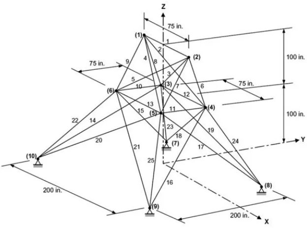
In this structure, shown in Figure 4, each node is connected to every other node by a member, except for members between the fixed support nodes 5, 6, 7, and 8. In this example, the modulus of elasticity and the material density of all members were 10,000 ksi and 0.1 lb/in.3, respectively. The 22 members were linked into seven groups, as follows: (1) A1 ~ A4, (2) A5 ~ A6, (3) A7 ~ A8, (4) A9 ~ A10, (5) A11 ~ A14, (6) A15 ~ A18, and (7) A19 ~ A22. The truss members were subjected to the stress limitations shown in Table 1. Also, displacement constraints of ±2.0 in. were imposed on all nodes in all directions. Three loading conditions described in Table 2 were considered, and a minimum member cross-sectional area of 0.1 in.2 was enforced.

41

Table 1. Member stress limitation for the 22-bar space truss.

Variables Compressive stress limitation (ksi)

Tensile stress limitation (ksi)

1 A1 ~ A4 24.0 36.0

2 A5 ~ A6 30.0 36.0

3 A7 ~ A8 28.0 36.0

4 A9 ~ A10 26.0 36.0

5 A11 ~ A14 22.0 36.0

6 A15 ~ A18 20.0 36.0

7 A19 ~ A22 18.0 36.0

Table 2. Loading condition for the 22-bar space truss.

Condition 3 Condition 2 Condition 1 Node PZ PY PX PZ PY PX PZ PY PX 35.0 0.0 -20.0 0.0 -5.0 -20.0 -5.0 0.0 -20.0 1 0.0 0.0 -20.0 0.0 -50.0 -20.0 -5.0 0.0 -20.0 2 0.0 0.0 -20.0 0.0 -5.0 -20.0 -30.0 0.0 -20.0 3 -35.0 0.0 -20.0 0.0 -50.0 -20.0 -30.0 0.0 -20.0 4

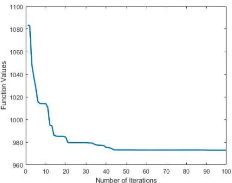
Figure 5 shows the convergence history of the best result obtained by WCA for 22-bar spatial truss. Results obtained for this structure are summarized in Table 3. It can be seen that WCA can find best global optimum compare to the other results.

42

Table 3. Optimal desig comparison for the 22-bar space truss.

Variables

Optimal cross-sectional areas (in.2₎

Sheu and Schmit [27]

Khan and Willmert [28]

Lee and Geem

[29] This work 1 A1 ~ A4 2.629 2.563 2.588 2.9784

2 A5 ~ A6 1.162 1.553 1.083 1.2400

3 A7 ~ A8 0.343 0.281 0.363 0.5262

4 A9 ~ A10 0.423 0.512 0.422 0.100

5 A11 ~ A14 2.782 2.626 2.827 3.3685

6 A15 ~ A18 2.173 2.131 2.055 1.6077

7 A19 ~ A22 1.952 2.213 2.044 1.2337

Weight (lb) 1024.80 1034.74 1022.23 972.872

Note: 1 in.2 _{= 6.452 cm}2_{, 1 lb = 4.45 N.}

4.2. Twenty-Five-Bar Spatial Truss

The 25-bar transmission tower space truss, shown in Figure 6, has been size optimized by many researchers. In this example, the material density is 0.1 lb/in.3 and modulus of elasticity is 10,000 ksi. This space truss was subjected to the two loading conditions shown in Table 4. The structure was required to be doubly symmetric about the x- and y-axes; this condition grouped the truss members as follows: (1) A1, (2) A2 ~ A5, (3) A6 ~ A9, (4) A10 ~ A11, (5) A12 ~ A13, (6) A14 ~ A17, (7) A18 ~ A21, and (8) A22 ~ A25. The truss members were subjected to the compressive and tensile stress limitations shown in Table 5. In addition, maximum displacement limitations of ±0.35 in. were imposed on every node in every direction. The minimum cross-sectional area of all members was 0.01 in.2.

43

Table 4. Loading condition for the 25-bar space truss.

Condition 2 Condition 1

Node

PZ

PY

PX

PZ

PY

PX

-5.0 10.0

1.0 -5.0 20.0 0.0

1

-5.0 10.0

0.0 -5.0 -20.0 0.0

2

0.0 0.0

0.5 0.0

0.0 0.0

3

0.0 0.0

0.5 0.0

0.0 0.0

6

Table 5. Member stress limitation for the 25-bar space truss.

Variables Grouped Compressive stress limitation (ksi)

Tensile stress limitation (ksi)

1 A1 35.092 40.0

2 A2 ~ A5 11.590 40.0

3 A6 ~ A9 17.305 40.0

4 A10 ~ A11 35.092 40.0

5 A12 ~ A13 35.092 40.0

6 A14 ~ A17 6.759 40.0

7 A18 ~ A21 6.959 40.0

8 A22 ~ A25 11.082 40.0

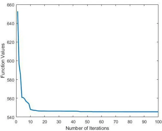
Figure 7 shows the convergence trend towards the optimum. Table 6. lists the optimal values of the eight size variables obtained by this research, and compares them with other results. As illustrated in Figure 7 WCA obtained the best solution at 45 iterations (4500 function evaluations) and it has fast convergence rate.

44

Table 6. Optimal desig comparison for the 25-bar space truss.

Variables Optimal cross-sectional areas (in.2₎

Khan and Willmert [28] Rizzi [30] Saka [31] Venkayya [32] This work

1 A1 0.01 0.01 0.01 0.028 0.01

2 A2 ~ A5 1.755 1.988 2.085 1.964 2.0338

3 A6 ~ A9 2.869 2.991 2.988 3.081 2.9755

4 A10 ~ A11 0.01 0.01 0.01 0.01 0.01

5 A12 ~ A13 0.01 0.01 0.01 0.01 0.01

6 A14 ~ A17 0.845 0.684 0.696 0.693 0.6835

7 A18 ~ A21 2.011 1.677 1.670 1.678 1.6440

8 A22 ~ A25 2.478 2.663 2.592 2.627 2.6743

Weight (lb) 553.94 545.16 545.23 545.49 545.069

Note: 1 in.2 _{= 6.452 cm}2_{, 1 lb = 4.45 N.}

4.3. Seventy-Two-Bar Spatial Truss

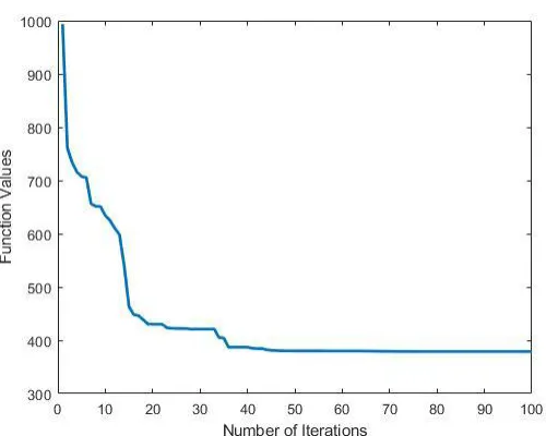
For the 72-bar space truss, shown in Figure 8, the material density and modulus of elasticity are 0.1 lb/in.3 and 10,000 ksi, respectively. The members are subjected to the stress limits of ±25 ksi. The uppermost nodes are subjected to the displacement limits of ±0.25 in. in both the x and y directions. The 72 structural members of this spatial truss are sorted into 16 groups using symmetry: (1) A1 ~ A4, (2) A5 ~ A12, (3) A13 ~ A16, (4) A17 ~ A18, (5) A19 ~ A22, (6) A23 ~ A30, (7) A31 ~ A34, (8) A35 ~ A36, (9) A37 ~ A40, (10) A41 ~ A48, (11) A49 ~ A52, (12) A53 ~ A54, (13) A55 ~ A58, (14) A59 ~ A66, (15) A67 ~ A70, and (16) A71 ~ A72. The minimum permitted cross-sectional area of each member is 0.10 in2, and the maximum cross-sectional area of each member is 4.00 in2. Table 7 lists the values and directions of the two load cases applied to the 72-bar spatial truss.

Table 7.Loading condition for the 72-bar space truss.

Condition 2 Condition 1 Node PZ PY PX PZ PY PX -5.0 0.0 0.0 -5.0 5.0 5.0 17 -5.0 0.0 0.0 0.0 0.0 0.0 18 -5.0 0.0 0.0 0.0 0.0 0.0 19 -5.0 0.0 0.0 0.0 0.0 0.0 20

45

Figure 8. 72-bar space truss.

46

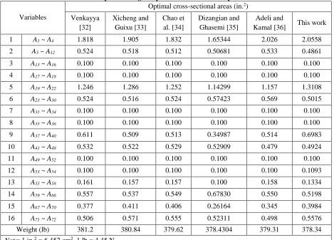
Table 8:Optimal desig comparison for the 72-bar space truss.

Variables

Optimal cross-sectional areas (in.2₎

Venkayya [32]

Xicheng and Guixu [33]

Chao et al. [34]

Dizangian and Ghasemi [35]

Adeli and

Kamal [36] This work

1 A1 ~ A4 1.818 1.905 1.832 1.65344 2.026 2.0558

2 A5 ~ A12 0.524 0.518 0.512 0.50681 0.533 0.4861

3 A13 ~ A16 0.100 0.100 0.100 0.100 0.100 0.100

4 A17 ~ A18 0.100 0.100 0.100 0.100 0.100 0.100

5 A19 ~ A22 1.246 1.286 1.252 1.14299 1.157 1.3108

6 A23 ~ A30 0.524 0.516 0.524 0.57423 0.569 0.5015

7 A31 ~ A34 0.100 0.100 0.100 0.100 0.100 0.100

8 A35 ~ A36 0.100 0.100 0.100 0.100 0.100 0.100

9 A37 ~ A40 0.611 0.509 0.513 0.34987 0.514 0.6983

10 A41 ~ A48 0.532 0.522 0.529 0.52909 0.479 0.4924

11 A49 ~ A52 0.100 0.100 0.100 0.100 0.100 0.100

12 A53 ~ A54 0.100 0.100 0.100 0.100 0.100 0.1093

13 A55 ~ A58 0.161 0.157 0.157 0.100 0.158 0.1334

14 A59 ~ A66 0.557 0.537 0.549 0.67830 0.550 0.5198

15 A67 ~ A70 0.377 0.411 0.406 0.26164 0.345 0.3984

16 A71 ~ A72 0.506 0.571 0.555 0.52311 0.498 0.5576

Weight (lb) 381.2 380.84 379.62 378.4304 379.31 378.34

Note: 1 in.2 _{= 6.452 cm}2_{, 1 lb = 4.45 N.}

5. Conclusions and Discussions

In this paper, three examples of spatial truss structures including a 22-bar space truss, a 25-bar space truss, and a 72-bar space truss were optimized. The trusses were optimized under stress and displacement constrains with water cycle algorithm (WCA). Results show that WCA could find better global optimum in comparison with other well-known optimization algorithms. Moreover, fast convergence rate to find the best solution and low number of function evaluation are considered as other advantages of WCA for optimizing of spatial trusses.

6. References

[1]- Ling-xi, Q., Wanxie, Z., Yunkang, S., and Jintong, Z., 1982, Efficient optimum design of

structures—program DDDU, Computer Methods in Applied Mechanics and Engineering, 30(2),

209-24.

[2]- Templeman, A. B., 1988, Discrete optimum structural design, Computers and Structures,

30(3), 511-518.

[3]- Hall, S. K., Cameron, G. E., and Grierson, D. E., 1989, Least-weight design of steel

47

[4]- Adeli, H., and Park, H. S., 1995, A neural dynamics model for structural optimization—

theory, Computers and structures, 57(3), 383-390.

[5]-Tzan, S. R., and Pantelides, C. P., 1996, Annealing strategy for optimal structural design,

Journal of Structural Engineering, 122(7), 815-827.

[6]- Deb, K., 2012, Optimization for engineering design: Algorithms and examples, PHI

Learning Pvt. Ltd.

[7]- Rao, S. S., and Rao, S. S., 2009, Engineering optimization: theory and practice, John Wiley

& Sons.

[8]-Nanakorn, P., and Meesomklin, K., 2001, An adaptive penalty function in genetic

algorithms for structural design optimization, Computers and Structures, 79(29), 2527-2539.

[9]- Sivaraj, R., and Ravichandran, T., 2011, A review of selection methods in genetic algorithm,

International Journal ofEngineering Science and Technology, 3, 3792-3797.

[10]- Salar, M., Ghasemi, M. R. and Dizangian, B. A., 2015, fast GA-based method for solving

truss optimization problems, International Journal of Optimization in Civil Engineering, 6(1),

101-114.

[11]- Das, S., and Suganthan, P. N., 2011, Differential evolution: A survey of the

state-of-the-art, Trans Evol Comput. IEEE, 15, 4-31.

[12]- Simon, D., 2008, Biogeography-based optimization, Trans Evol Comput, IEEE, 12,

702-713.

[13]- Kirkpatrick, S., Gelatt, C. D., and Vecchi, M. P., 1983, Optimization by simulated

annealing, Science, 220 (4598), 671-680.

[14]- Kaveh, A. and Talatahari, S., 2010, Optimal design of skeletal structures via the charged

system search algorithm, Structure Multidisciplinary Optimization, 41(6), 893-911.

[15]- Nouhi, B., Talatahari, S., Kheiri, H., and Cattani, C., 2013, Chaotic charged system search

with a feasible-based method for constraint optimization problems, Mathematical Problem

Engineering, Article ID 391765, 8 pages.

[16]- Kaveh, A., and Mahdavai, V. R., 2014, Colliding bodies optimization: A novel

meta-heuristic method, Computer Structure, 139, 18-27.

[17]- Eberhart, R. C., and Kennedy, J. A., 1995, new optimizer using particle swarm theory,

Proceedings of the Sixth International Symposium on Micro Machine and Human Science,

Nagoya, Japan.

[18]- Geem, Z. W., 2009, Harmony Search Algorithms for Structural Design, Springer Verlag.

[19]- Karaboga, D., Gorkemli, B., Ozturk, C., and Karaboga, N. A., 2014, comprehensive survey:

artificial bee colony (ABC) algorithm and applications, Artificial Intelligence Review, 42,

21-57.

[20]- Yang, X. S., and Deb, S., 2014, Cuckoo search: recent advances and applications, Neural

ComputingApplications, 24, 169-174.

[21]- Yang, X. S., 2010, Firefly algorithm, stochastic test functions and design optimization,

International Journal ofBio-inspired Computing, 2(2), 78-84.

[22]- Gandomi, A. H., and Alavi, A. H., 2012, Krill herd: a new bio-inspired optimization

48

[23]- Yang, X. S., 2010, A new metaheuristic bat-inspired algorithm, in: Nature Inspired

Cooperative Strategies for Optimization (NISCO 2010) (Eds JR Gonzalez et al), Studies in Computational Intelligence, Springer Berlin, 284, Springer, 65-74.

[24]- Eskandar, H., Sadollah, A., Bahreininejad, A., and Hamdi, M., 2012, Water cycle algorithm

-A novel metaheuristic optimization method for solving constrained engineering optimization

problems, Computing Structure, 110-111,151-166.

[25]- Eskandar, H., Sadollah, A., and Bahreininejad, A., 2013, Weight optimization of truss

structures using water cycle algorithm, Iran University of Science and Technology, 3(1),

115-129.

[26]- Lee, K. S., and Geem, Z. W., 2004, A new structural optimization method based on the

harmony search algorithm, Computing Structure, 82, 781–798.

[27]- Sheu, C. Y., and Schmit, L. A., 1972, Minimum weight design of elastic redundant trusses

under multiple static loading conditions, AIAA Journal, 10(2), 155-162.

[28]- Khan, M. R., Willmert, K. D., and Thornton, W. A., 1979, An optimality criterion method

for large-scale structures, AIAA journal, 17(7), 753-761.

[29]- Lee, K. S., and Geem, Z. W., 2004, A new structural optimization method based on the

harmony search algorithm, Computers and structures, 82(9),781-798.

[30]- Rizzi, P., 1976, Optimization of multi-constrained structures based on optimality

criteria, InProc. AIAA/ASME/SAE 17th Structures, Structural Dynamics and Materials

Conference (pp. 448-462).

[31]- Saka, M. P., Optimum design of pin-jointed steel structures with practical applications,

Journal of Structural Engineering,116(10), 2599-2620.

[32]- Venkayya, V. B., 1971, Design of optimum structures, Computers and Structures,

1;1(1-2), 265-309.

[33]- Xicheng, W., and Guixu, M., 1992, A parallel iterative algorithm for structural

optimization, Computer Methods in Applied Mechanics and Engineering, 96(1), 25-32.

[34]- Chao, N. H., Fenves, S. J., Westerberg, A. W., 1981, Application of a reduced quadratic

programming technique to optimal structural design. Carnegie-Mellon University Pittsburgh

PA.

[35]- Dizangian, B., and Ghasemi, M. R., 2015, Ranked-based sensitivity analysis for size

optimization of structures, Journal of Mechanical Design, 137(12), 121-142.

[36]-Adeli, H., and Kamal, O., 1986, Efficient optimization of space trusses, Computers and