DEMOGRAPHIC RESEARCH
A peer-reviewed, open-access journal of population sciences
DEMOGRAPHIC RESEARCH
VOLUME 31, ARTICLE 19, PAGES 553–592
PUBLISHED 2 SEPTEMBER 2014
http://www.demographic-research.org/Volumes/Vol31/19/
DOI: 10.4054/DemRes.2014.31.19
Research Article
A matrix approach to the statistics of longevity
in heterogeneous frailty models
Hal Caswell
c
2014 Hal Caswell.
1 Introduction 554
2 The matrix formulation of the gamma-Gompertz model 556
2.1 Constructing transition matrices and the vec-permutation model 558
2.2 The absorbing Markov chain 559
3 Analysis of the model 559
3.1 The marginal survival and mortality functions 560
3.2 The marginal fundamental matrix 560
3.3 Longevity, variation, and disparity 561
3.4 Projecting the distributions of age, frailty, and mortality 562
4 An example: Swedish females 564
4.1 Statistics of longevity 565
4.2 Dynamics of frailty 566
4.3 Effects of the G-G parameters 567
4.4 Numerical reliability 571
5 Generalizations and extensions of the model 572
5.1 Models for baseline mortality 573
5.2 Models for the effects of frailty 574
5.3 Models for the distribution of frailty 575
5.4 Models for the dynamics of frailty 575
5.5 Some animal mortality patterns 577
6 Heterogeneous frailty vs. individual stochasticity: partitioning variance in longevity 578
7 Conclusions 580
7.1 Some pleasant properties of the matrix formulation 581
8 Acknowledgments 582
References 584
Appendix A: Gamma-Makeham and Gamma-Siler models 588
A matrix approach to the statistics of longevity in heterogeneous
frailty models
Hal Caswell1
Abstract
BACKGROUND
The gamma-Gompertz model is a fixed frailty model in which baseline mortality in-creases exponentially with age, frailty has a proportional effect on mortality, and frailty at birth follows a gamma distribution. Mortality selects against the more frail, so the marginal mortality rate decelerates, eventually reaching an asymptote. The gamma-Gompertz is one of a wider class of frailty models, characterized by the choice of baseline mortality, effects of frailty, distributions of frailty, and assumptions about the dynamics of frailty.
OBJECTIVE
To develop a matrix model to compute all the statistical properties of longevity from the gamma-Gompertz and related models.
METHODS
I use the vec-permutation matrix formulation to develop a model in which individuals are jointly classified by age and frailty. The matrix is used to project the age and frailty dy-namics of a cohort and the fundamental matrix is used to obtain the statistics of longevity.
RESULTS
The model permits calculation of the mean, variance, coefficient of variation, skewness and all moments of longevity, the marginal mortality and survivorship functions, the dy-namics of the frailty distribution, and other quantities. The matrix formulation extends naturally to other frailty models. I apply the analysis to the gamma-Gompertz model (for humans and laboratory animals), the gamma-Makeham model, and the gamma-Siler model, and to a hypothetical dynamic frailty model characterized by diffusion of frailty with reflecting boundaries.
The matrix model permits partitioning the variance in longevity into components due to heterogeneity and to individual stochasticity. In several published human data sets,
1Hal Caswell, Institute for Biodiversity and Ecosystem Dynamics, University of Amsterdam, PO Box 94248,
heterogeneity accounts for less than 10% of the variance in longevity. In laboratory pop-ulations of five invertebrate animal species, heterogeneity accounts for 46% to 83% of the total variance in longevity.
1. Introduction
The gamma-Gompertz (hereafter, G-G) model is one of a class of models that investigate the effects of hidden heterogeneity — heterogeneity that is either unobservable or un-observed — on mortality rates. It calculates various consequences of that heterogeneity for the dynamics of cohorts (e.g. Vaupel, Manton, and Stallard 1979; Vaupel and Yashin 1985; Yashin, Iachine, and Begun 2000; Vaupel 2010; Wienke 2010; Missov 2013). I refer to this heterogeneity asfrailty, making no assumptions about its causes. The goal of this paper is to present a matrix formulation that permits easy computation of all the properties of the G-G and other frailty models.
Frailty models can be characterized by their components:
1. the baseline mortality rate,
2. the effects of frailty on the baseline mortality rate, 3. the dynamics of individual frailty over time, and 4. the initial distribution of frailty.
The baseline mortality rate in the G-G model is the Gompertz model, in which mor-tality increases exponentially with aget,
µ(t) =aebt. (1)
Frailty affects mortality as a proportional hazard. IfZ(a non-negative random variable) denotes frailty, andzits realization, then the mortality of an individual with frailtyzat agetis
µ(z, t) =zµ0(t) (2)
whereµ0(t)is the baseline mortality schedule. The frailtyzis a fixed property of the individual, and the initial distribution of frailty is a gamma distribution.
Many other frailty models can be created by changing one or more of these four components. As we will see, the matrix formulation applies directly to all of them. Other pleasing properties of the matrix formulation will be discussed in Section 7.
The more frail individuals tend to die sooner, and the cohort is progressively dominated by individuals of lower frailty.
To summarize some well known facts about the G-G model (Wienke 2010; Vaupel and Missov forthcoming), because frailty is unobserved, observations on the cohort reveal not the individual mortality schedules, but rather the marginal mortality rate
µ∗(t) = Z
π(z, t)µ(z, t)dz (3)
whereπ(z, t)is the distribution of frailty at aget. The survivorship function of an indi-vidual of frailtyzis
S(z, t) = exp
−
Z t
0
µ(z, x)dx
(4)
and the marginal survivorship function of the cohort is
S∗(t) = Z
π(z,0)S(z, t)dz. (5)
The distribution of frailty at agetis obtained by multiplying the initial probability density for frailtyzby the probability that an individual with frailityzsurvives to aget, and then scaling the result by dividing by the integral:
π(z, t) =R π(z,0)S(z, t)
π(z,0)S(z, t)dz. (6)
The G-G model assumes that frailty is a fixed individual property and that the cohort begins life with frailty distributed according to a gamma distribution,z ∼gamma(k, λ) with shape parameterkand scale parameter2λ. The mean and variance ofzareE(z) =
k/λ and V(z) = k/λ2. Thus, when E(z) = 1, the distribution is given by
gamma 1/σ2,1/σ2
.
2The probability density function is
gamma(k, λ) = 1
Γ(k)λk z
k−1e−z/λ. (7)
Note that two parameterizations of the gamma distribution are widely used. Equation (7) is common in
demog-raphy. MATLABuses the parameterization
gamma(k, θ)
wherekis a shape parameter andθis a rate parameter. In this parameterization,E(z) =kθandV(z) =kθ2.
Thus in MATLABthe distribution with mean equal to 1 is gamma 1/σ2, σ2
The marginal mortality rate (3) for the G-G model is a sigmoid function of age,
µ∗(t) = ae bt
1 + aσb2 (ebt−1) (8)
(Yashin, Vaupel, and Iachine 1994), converging to an asymptote atb/σ2astgets large.
Thus, the G-G model is an attractive explanation for the widely observed pattern of de-celerating increase in mortality with age, in both humans and other species (e.g., Vaupel et al. 1998; Horiuchi 2003; Vaupel 2010; Missov and Finkelstein 2011).
Although it is simple to state, and widely used, deriving the consequences of the G-G model is mathematically challenging. Only recently has Missov (2013) obtained an expression for life expectancy at birth, by integrating the survivorship function (5). The result, a function of the Gompertz parametersaandb and the gamma distribution parameterskandλ, is
e0(a, b, k, λ) = 1
bk 2F1
k,1;k+ 1; 1− 1 bλ
(9)
where the function2F1(·)is the Gaussian hypergeometric function.3
Life expectancy, however, is only one of many demographic properties implied by a mortality model. My goal here is to present a matrix formulation that provides not only the mean, but all the moments of longevity, various measures of life disparity, and the full dynamics of the joint distribution of age and frailty. It will become apparent from the construction of this model that it applies equally to a much broader class of frailty models, and I will present examples.
The organization of this paper is as follows. Section 2 derives the matrix model, using methods developed for populations in which individuals are jointly classified by age and stage. Section 3 derives the fundamental matrix, the moments of longevity, the distri-bution of age at death, and other indices from the matrix model including (Section 3.4) the dynamics of the frailty distribution over the life of the cohort. Section 4 analyzes an example, using parameter estimates for Swedish females taken from Missov (2013). Section 5 discusses some interesting generalizations, with examples. Section 6 uses the model to partition variance in longevity into components due to individual stochasticity and heterogeneous frailty. Section 7 concludes by presenting a protocol for computation and discusses further extensions.
3For more on the Gaussian hypergeometric distribution, see Abramowitz and Stegun (1965, 15.1.1) or the
2. The matrix formulation of the gamma-Gompertz model
Notation. In what follows, matrices are denoted by upper-case boldface letters, and vectors by lower-case boldface letters. Where necessary, the dimensions of matrices and vectors are denoted by subscripts; thusIn is an identity matrix of ordernand1n is a
n×1vector of ones. The vectoreiis theith unit vector. The diagonal matrix withxon the diagonal and zeros elsewhere is denotedD(x). The symbol◦denotes the Hadamard, or element-by-element product. The symbolkxkdenotes the 1-norm of the vectorx. The number of age classes isωand the number of frailty groups isg.
The matrix G-G model is an age-stage classified model in which stages correspond to frailty classes. Age-stage classified matrix models have been analyzed in other contexts by Caswell (2009, 2011, 2012) and Caswell and Salguero-G´omez (2013). The model is created using the vec-permutation formalism (Hunter and Caswell 2005) and analyzed using absorbing Markov chain theory (Caswell 2006, 2009, 2013)
To construct the matrix G-G model, let us introduce some notation. Age is described by a set of discrete age classes1, . . . , ω. The baseline mortality rates are contained in a vectorµ0of dimensionω×1. For the Gompertz mortality model, the baseline mortality rate vector is
µ0=a
e0b e1b e2b .. .
e(ω−1)b
(10)
Frailty is described by a set of g discrete frailty classes; the frailty values of these classes are given by ag×1vectorz. To create the frailty classes, first specify a maximum frailty, where the cumulative gamma distribution reaches some high value; say, 0.9999. Since very high values of frailty are rapidly eliminated, this end of the distribution is, in practice, not very important. Then specify a minimum value of frailty as some very small number; for the applications reported here, a value on the order of10−7was adequate.
Since individuals with very low frailty will persist for a long time in the population, it is important thatzminbe small.
Experience suggests that logarithmically spaced values betweenzminandzmaxwork well, because they provide more detail in the frailty distribution at the low end, precisely where individuals will persist the longest. An alternative is to evenly divide the inverse of the cumulative distribution function, so that values are most closely spaced where the concentration of initial probability is greatest. Given the vectorzof frailty classes, the vector of mortality rates by age, for frailty classi, is
The distribution of individuals among frailty classes at agetis given by the vector π(t); the initial frailty distribution of the cohort is given byπ(0). In the matrix G-G model,π(0)is a discrete gamma distribution with mean of 1 and a specified variance.
2.1 Constructing transition matrices and the vec-permutation model
To construct the age-stage model, define a survival matrix for each frailty class, and a matrix of frailty transitions for each age class, as follows.
1. Create a survival matrixUifor each frailty classi. It contains survival probabilities on the first subdiagonal and zeros elsewhere, and is of dimensionω×ω.
Ui=
0 0 · · · 0
e−µ(zi,0) 0 · · · 0
..
. . .. ...
0 · · · e−µ(zi,ω−1) 0 (12)
2. Create a matrixDjdescribing transitions among frailty classes for each age class
j. In the gamma-Gompertz model, frailty does not change, soDj =Igfor allj. 3. Create block-diagonal matricesUandDby placing theUi (respectively,Dj) on
the diagonal with zeros elsewhere. Both matrices are of dimensionωg×ωg.
U=
U1 · · · 0
..
. . .. ... 0 · · · Ug
D=
D1 · · · 0
..
. . .. ... 0 · · · Dg
(13)
In the gamma-Gompertz model,D=Iωg.
The state of the cohort at agetis given by a vectorn˜(t), which is derived from the array
N(t) =
n11 · · · n1g ..
. ...
nω1 · · · nωg
(14)
that describes the abundance of all age-frailty categories. The population vector is
˜
n=vecNT
that is, ˜ n= n11 .. .
n1g .. .
nω1
.. . nωg (16)
Theith block of entries inn˜ contains a sub-vector giving the abundance of the frailty classes within age classi.
The joint age-frailty composition of the cohort is projected as
˜
n(t+ 1) = ˜Un˜(t) (17)
where the projection matrix is
˜
U=DKUKT
(18)
In equation (18),K(to be more precise,Kω,g) is the vec-permutation matrix, or commu-tation matrix (Magnus and Neudecker 1979; Henderson and Searle 1981). See (Hunter and Caswell 2005; Caswell 2012) for more about models of the form (18).
Because frailty is fixed in the gamma-Gompertz model,U˜ reduces toU˜ =KUKT.
However, it is good practice to retain the matrixDas a reminder of its potential use when frailty is dynamic rather than static.
2.2 The absorbing Markov chain
The matrixU˜ in (17) is the transient matrix of an absorbing Markov chain (Feichtinger 1971; Caswell 2001, 2006, 2009; van Raalte and Caswell 2013). The transition matrix of this chain is
P= ˜ U 0 ˜ M I ! (19)
whereM˜ is a mortality matrix describing the transitions from transient (i.e., living) states to absorbing (i.e., dead) states. The fundamental matrix of the chain is
˜
N=Iωq−U˜ −1
(20)
with dimensionωg×ωg. The(i, j)entry ofN˜ is the expected number of visits to state
distribution. From the fundamental matrix we can compute all the statistics of the cohort survival properties. We turn now to these analyses.
3. Analysis of the model
The fundamental matrixN˜ of the joint chain contains all the information necessary to de-rive the marginal survival functions∗(a vector of dimensionω×1) and the corresponding marginal fundamental matrixN∗(of dimensionω×ω).
3.1 The marginal survival and mortality functions
To obtain the marginal dynamics of the cohort age distribution, first average the columns ofN˜ over the initial frailty distribution. If, as in the gamma-Gompertz case, the initial frailty distribution has positive support only in the first age class, the result is
˜s= ˜N
e1⊗π(0)
.
This column vector gives the expectation, over π(0), of the number of visits to each age-frailty state by an individual in the first age class.
Next, sum the rows of the vector˜swithin each frailty class to obtain the marginal mean number of visits to each age class for an individual in the initial cohort. Because the underlying demographic model is age-classified, a transient state (i.e., an age class)
can be visited at most once; hence the mean number of visits to age classiis the proba-bility of visiting age classi, which is the survivorship to age classi. Thus the marginal survivorship functions∗is
s∗ = Iω⊗1Tg
˜s (21)
= Iω⊗1Tg
˜
N[e1⊗π(0)] (22)
The marginal mortality rate vectorµ∗is given by the difference in the log of subse-quent terms ofs∗,
µ∗i =−log s∗
i+1 s∗
i
3.2 The marginal fundamental matrix
The fundamental matrixN˜ gives the number of visits to each age-frailty class. We need the marginal fundamental matrixN∗, which gives the expected number of visits to each age class. To obtainN∗, note that the vectors∗is the first column ofN∗, and that the full matrix is
N∗=
s∗1 0 0 · · · 0
s∗2 s∗2
s∗
2 0 · · · 0
s∗3 s∗3
s∗
2
s∗
3
s∗
3 · · · 0
s∗4 s∗4
s∗
2
s∗
4
s∗
3 · · · 0 ..
. ... ... · · · 1 (24)
(Keyfitz and Caswell 2005, Eq. 10.5.4)4, which can be written
N∗=hs∗1T
sD(s
∗)−1i
◦Y (25)
whereY is a lower triangular matrix with ones on and below the diagonal and zeros elsewhere.
3.3 Longevity, variation, and disparity
Many statistics of longevity can be obtained from the marginal fundamental matrixN∗
(e.g., Caswell 2001, 2006, 2009, 2013; van Raalte and Caswell 2013; Engelman, Caswell, and Agree 2014). These statistics describe the marginal results for the cohort starting with the initial frailty distributionπ(0), including:
1. The moments of the number of visits to each of the transient states. Because tran-sient states (age classes) in an age-classified model can be visited no more than once, these moments may be less interesting in the G-G model than in models with more complicated stage structure. LettingN∗i be the matrix of theith moments of the number of visits,N∗1is given by (24), and the higher moments include
N∗2 = 2N∗dg−I
N∗1 (26)
N∗3 = h6 N∗dg2
−6N∗dg+IiN∗1 (27)
N∗4 = h24 N∗dg3−36 Ndg∗ 2+ 14N∗dg−IiN∗1. (28)
whereN∗dgis a diagonal matrix with the diagonal elements ofN∗1on the diagonal
and zeros elsewhere (e.g., Caswell 2006, 2009, 2013); for a mathematical source see Iosifescu (1980).
2. The moments and statistics of longevity. Longevity is equivalent to the time until absorbtion in one of the absorbing states. The vectorη1of mean longevities (i.e., life expectancies) of each age class is given by the column sums ofN∗, and subse-quent moments are as follows, whereηiis the vector ofith moments of longevity:
ηT
1 = 1
T
ωN
∗ (29)
ηT
2 = η
T
1(2N∗−I) (30)
ηT
3 = η
T
1
h
6 (N∗)2−6N∗+Ii (31)
ηT
4 = η
T
1
h
24 (N∗)3−36 (N∗)2+ 14N∗−Ii. (32)
(Caswell 2006, 2009, 2013). These moments provide a complete set of longevity statistics, including the variance, standard deviation, coefficient of variation, and skewness of longevity:
V (η) = η2−η1◦η1 (33)
SD(η) = pV(η) (34)
CV (η) = D(η1)−1SD(η) (35)
Sk(η) = D(V(η))−3/2
η3−3η1◦η2+ 2η1◦η1◦η1
(36)
3. The joint and marginal distributions of age and stage at death. Because the matrix G-G model is an age-stage structured model, the joint and marginal distributions of age and frailty class at death are obtained using the mortality matrixM˜ in (19). IfM˜ is created by defining absorbing states corresponding to the age and frailty
class at death, thenM˜ =D1T
ωg−1TωgU˜
. Then columnjof the matrix
˜
B= ˜MN˜ (37)
gives the joint distribution of age and frailty at death, conditional on reaching the age-frailty combination in columnj(Caswell 2012).
Averaging the firstgcolumns ofB˜ over the initial frailty distribution gives a vector ˜
φ containing the distribution of age and frailty at death of a cohort with initial frailty distributionπ(0):
˜
φ= ˜Bhe1⊗π(0)
i
The marginal distributions of age and of frailty at death are obtained by summing over the appropriate rows ofφ˜,
φ∗age = Iω⊗1Tg ˜
φ (39)
φ∗frailty = (1Tω⊗Ig) ˜φ (40)
3.4 Projecting the distributions of age, frailty, and mortality
The population vector giving the abundance by age and frailty class is projected by the matrixU˜ in (18):
˜
n(t+ 1) = ˜Un˜(t) (41)
If, as in the G-G model, the initial cohort has support only in the first age class, with distributionπ(0), thenn˜(0) = (eT
1⊗Ig)π(0).
Letp˜(t)be the vector giving theproportionalage-frailty distribution at timet. It is given by
˜
p(t+ 1) = ˜ Up˜(t)
kU˜p˜(t)k, (42)
withp˜(0) = ˜n(0)/kn˜(0)k.
The marginal age vector and the marginal proportional age distribution vector are obtained by summing over frailty classes within age classes, as was done in (39) for the death distribution. They are given by
n∗(t) = Iω⊗1Tg
˜
n(t) (43)
p∗(t) = Iω⊗1Tg
˜
p(t) (44)
The marginal frailty vector and the marginal proportional frailty distribution are obtained by summingn˜andp˜over age within each frailty class, as was done in (40) for the death distribution:
m∗(t) = (1T
ω⊗Ig) ˜n(t) (45)
π(t) = (1T
ω⊗Ig) ˜p(t) (46)
The marginal distribution vectorπ(t)corresponds to the frailty distribution as a function of age given in (6). Fromπ(t), the statistics, particularly the mean and variance, of frailty and of any quantity that is a function of frailty, can be calculated, to quantify the effects of selection as a function of age. For example, the mean frailty at agetis given byzTπ(t),
and the second moment is given by(z◦z)T
marginal mortality rateµ∗in (23) is the first moment; we can calculate all the moments, and hence such statistics as the variance, CV, skewness, etc. as follows.
First, use the frailty model to create hazard matricesHmcontaining themth powers of the mortality rates,
Hm=
µm11 · · · µm1g ..
. ...
µmω1 · · · µmωg
(ω×g) (47)
The form ofHmwill depend on the chosen frailty model; in the special case of the G-G model,
Hm= (µ0z
T)◦ · · · ◦(µ
0z
T)
| {z }
mtimes
(48)
whereµ0is the baseline mortality vector andzthe vector of frailty values for thegfrailty classes.
Then, create a matrix Π containing, as columns, the frailty distributions obtained from (46),
Π=hπ(0)· · ·π(ω−1)i (g×ω) (49)
The vector containing the mth moments of the marginal mortality is the diagonal of
HmΠ,
µ∗m = diagonal ofHmΠ (50)
= hI◦(HmΠ) i
1 (51)
4. An example: Swedish females
An example of the calculations is provided by using the G-G parameters a, b, and k
estimated by Missov (2013) from period mortality data on Swedish females from 1891 to 2010. I used these parameters, for the arbitrarily selected year 1950, to create the matricesUandD(ˆa= 0.0340,ˆb= 0.1200,ˆk= 8.2300). Calculations were carried out
withω= 150age classes andg= 100logarithmically spaced frailty classes. A MATLAB program to carry out these calculations is available in the Supplementary Material to this paper.
Figure 1: Gamma-Gompertz mortality rateµ(t)as a function of age,t. Straight black lines show the age-specific mortality rates for a few of the frailty classes in the model. The curved red line shows the marginal hazardµ∗(t). Parameters for Swedish females as reported in Missov (2013) for the year 1950
0 50 100 150
10−15 10−10 10−5 100 105
Age
Mortality rate
4.1 Statistics of longevity
Figure 2: Statistics of longevity for the gamma-Gompertz model, as a function of age, using parameters reported in Missov (2013) for the year 1950. (a) Life expectancy. (b) Standard deviation of longevity. (c) Coefficient of variation of longevity. (d) Skewness of longevity. This and all subsequent figures, unless otherwise noted, computed withg= 100andω= 150
(a) Life expectancy
0 20 40 60 80 100 120
0 10 20 30 40 50 60 70 80
Age
Life expectancy
(b) Standard deviation of longevity
0 20 40 60 80 100 120
0 2 4 6 8 10 12
Age
SD of longevity
(c) CV of longevity
0 20 40 60 80 100 120
0.1 0.2 0.3 0.4 0.5 0.6 0.7 0.8
Age
CV of longevity
(d) Skewness of longevity
0 20 40 60 80 100 120
−1 −0.5 0 0.5 1 1.5 2 2.5
Age
Skewness of longevity
4.2 Dynamics of frailty
known to remain constant with age in the G-G model (Wienke 2010, p. 75). In the matrix calculation, it is very nearly constant, increasing slightly at about age 75.
Figure 3: Changes due to selection in the distribution of frailty, and in the mean, CV, and skewness of that distribution, over the life of a cohort. Parameters for Swedish females, as reported in Missov (2013) for the year 1950
(a) Frailty distribution
0 0.5 1 1.5 2 2.5 3
0 1 2 3 4 5 6
Frailty
Density
Age=1 90 100 110
(b) Mean frailty
0 20 40 60 80 100 120
0 0.2 0.4 0.6 0.8 1
Age
Mean frailty
(c) Standard deviation of frailty
0 20 40 60 80 100 120
0 0.05 0.1 0.15 0.2 0.25 0.3 0.35
Age
SD fraility
(d) CV of frailty
0 20 40 60 80 100 120
0.34 0.345 0.35 0.355 0.36
Age
CV fraility
4.3 Effects of the G-G parameters
Figure 4: Statistics of longevity for the gamma-Gompertz model, using parameters reported in Missov (2013) for Swedish females in 1950, as a function of the Gompertz parametera
(a) Life expectancy
100−8 10−6 10−4 10−2
20 40 60 80 100 120 Gompertz a Expected longevity 0 30 60
(b) Standard deviation of longevity
100−8 10−6 10−4 10−2
2 4 6 8 10 12 Gompertz a SD longevity 0 30 60
(c) CV of longevity
10−8 10−6 10−4 10−2
0 0.1 0.2 0.3 0.4 0.5 0.6 0.7 0.8 Gompertz a CV longevity 0 30 60
(d) Skewness of longevity
10−8 10−6 10−4 10−2
−1.5 −1 −0.5 0 0.5 1 1.5 2 Gompertz a Skew longevity 0 30 60
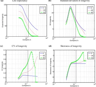
Figure 5: Statistics of longevity for the gamma-Gompertz model, using parameters reported in Missov (2013) for Swedish females in 1950, as a function of the Gompertz parameterb, for ages 0, 30, and 60 years
(a) Life expectancy
100−2 10−1 100
50 100 150
Gompertz b
Expected longevity
0 30 60
(b) Standard deviation of longevity
10−2 10−1 100
0 5 10 15 20
Gompertz b
SD longevity
0 30 60
(c) CV of longevity
10−2 10−1 100
0 0.1 0.2 0.3 0.4 0.5 0.6 0.7
Gompertz b
CV longevity
0 30 60
(d) Skewness of longevity
10−2 10−1 100
−8 −6 −4 −2 0 2 4
Gompertz b
Skewness of longevity
0 30 60
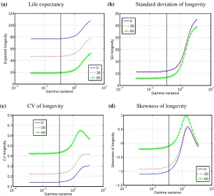
Figure 6: Statistics of longevity at ages 0, 30, and 60 years for the gamma-Gompertz model as a function of the variance in the gamma distribution of frailty (equal to1/k). Parameters as reported in Missov (2013) for Swedish females in 1950. The vertical lines indicate the observed value of variance
(a) Life expectancy
10−4 10−2 100 102
0 20 40 60 80 100 120 Gamma variance Expected longevity 0 30 60
(b) Standard deviation of longevity
10−4 10−2 100 102
5 10 15 20 25 30 35 Gamma variance SD longevity 0 30 60
(c) CV of longevity
10−4 10−2 100 102
0.1 0.2 0.3 0.4 0.5 0.6 0.7 0.8 Gamma variance CV longevity 0 30 60
(d) Skewness of longevity
10−4 10−2 100 102
−1.5 −1 −0.5 0 0.5 1 Gamma variance
Skewness of longevity
0 30 60
The effects of changes in the varianceσ2= 1/kof the initial frailty distributionπ(0)
are shown in Figure 6. Expected longevity is relatively insensitive toσ2until it becomes
much higher than that observed for Swedish females, at which point the mean, variance, and coefficient of variation of longevity all begin to increase with σ2. The skewness
4.4 Numerical reliability
Based on his results using the Gaussian hypergeometric function (9), Missov (2013) re-ports a life expectancy of 77.29 years for Swedish females in 1950. Evaluating his for-mula with the Gaussian hypergeometric function as implemented in MATLABor in Wol-fram Alpha gives a result of 76.22 years. The matrix calculation yields 77.23 years or, when adjusted by 0.5 years to correspond to a trapezoidal integration of the survival func-tion, 76.73 years. The differences among the various implementations of the calculation are small (Table 1).
Table 1: Comparison of life expectancy results from Missov (2013), from this paper, and from Missov’s theorem implemented in MATLABand calculated using Wolfram Alpha. The adjusted value from this paper has had 0.5 years subtracted to make the result directly comparable to a trapezoidal computation of the integral ofS∗(t). For the matrix calculations,ω= 150andg= 100
Source Expected longevity
Missov (2013) 77.29
Missov via Matlab 76.22
Missov via Wolfram 76.22
Matrix method 77.23
Matrix method (adjusted) 76.73
Because the matrix calculation is a discrete model, the results are influenced by the number of frailty classesgand the number of age classesωincluded in the model. The number of frailty classes determines how closely π(0) can approximate a gamma dis-tribution, and the ability ofπ(t)to capture the distribution of frailty at late ages when selection has been operating for a long time. The number of age classes determines the extent to which the longevity statistics are influenced by the death of all remaining indi-viduals at ageω, which is not part of the G-G model, but must appear in any finite state approximation.
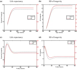
Figure 7 shows the effect ofωand ofgon the expectation and the standard deviation of longevity. For this example, choosingω >100andg >40provides reliable estimates of both the mean and the variation of longevity for this data set. Too small a value ofω
Figure 7: Effect of the number of age classes (ω) and the number of frailty classes (g) on the estimates of life expectancy and the standard deviation of longevity, at ages 0 and 50. (a) and (b) show the effects of age classes, withg= 100. (c) and (d) show the effect of the number of frailty classes, withω= 150
(a) Life expectancy
60 80 100 120 140 160
65 70 75 80 Age classes Expected longevity
60 80 100 120 140 16015 20 25 30
Age=0 50
(b) SD of longevity
60 80 100 120 140 160
5 6 7 8 9 10 11 12 Age classes SD longevity
60 80 100 120 140 1603 4 5 6 7 8 9 10 Age=0 50
(c) Life expectancy
10 20 30 40 50
75 76 77 78 79 Frailty classes Expected longevity
10 20 30 40 5026
27 28 29 30 Age=0 50
(d) SD of longevity
10 20 30 40 50
10.5 11 11.5 12 12.5 Frailty classes SD longevity
10 20 30 40 509
9.5 10 10.5 11 Age=0 50
5. Generalizations and extensions of the model
5.1 Models for baseline mortality
The baseline mortality scheduleµ0is used to create the frailty-specific mortality sched-ulesµiin equation (11). These schedules are used to create the matricesUithat appear in (13). The Gompertz model is only one possible choice of a baseline schedule. Here, I examine some alternatives; the results, in the same format as Figures 2, 3, and 4–6 are collected in Appendix A.
The Gompertz-Makeham model
µ(x) =aebx+c, (52)
is obtained by adding an age-independent morality hazardcto the Gompertz model. The gamma-Makeham model results from incorporating a porportional frailty effect
µi=zi aebi+c (53)
where thezihave a gamma distribution at age 0.
Modifyingµ0in equation (11) transforms the G-G model to the gamma-Makeham model, with
µ0=
e0b .. .
e(ω−1)b
+c
1 .. . 1
(54)
All analyses of the gamma-Makeham model then follow fromN˜, computed fromµ(z), just as with the G-G model.
Zarulli et al. (2013) estimated the parameters in the gamma-Makeham model as part of an analysis of the effects of education on the mortality of male and female cohorts in Turin, Italy, from 1971 to 2007. I analyzed their data for the baseline cohort of women, for which AIC calculations indicated that the gamma-Makeham model was much more well-supported by the data than the G-G model (Zarulli et al. 2013). Figure A.1 shows the expectation, standard deviation, CV, and skewness of remaining longevity as a function of age. The patterns are qualitatively similar to the gamma-Gompertz results for Swedish females (Figure 2). Selection reduces the mean and the standard deviation of frailty as age approaches 100, and the log of the marginal mortality rate increases with age in a sigmoid fashion (Figure A.2).
There is no reason to stop at the gamma-Makeham model. Gage (1998) and Engel-man, Canudas-Romo, and Agree (2013) have added gamma-distributed frailty to the Siler model for mortality
analysis of the gamma-Siler model requires only substituting this expression forµ0for
the gamma-Gompertz mortality function in (10).
Engelman, Canudas-Romo, and Agree (2013) estimated parameters of a gamma-Siler model for cohorts of Swedish females born from 1875–1916. Here I show results for the 1900 cohort. The expectation, standard deviation, CV, and skewness of remaining longevity are shown as functions of age in Figure A.3. The patterns differ from those of the G-G and gamma-Makeham models mainly in that they show the effects of the infant mortality term. This effect is also apparent in the marginal mortality function (Fig-ure A.4c) which declines sharply after birth, remains low, and then increases, eventually reaching a plateau at older ages.
These examples use parametric functions for the baseline mortality schedule, but they can easily be extended to semiparametric or nonparametric estimates. The estimated mortality function simply needs to be incorporated into the matricesUi.
5.2 Models for the effects of frailty
In the G-G model, frailty affects mortality as a proportional hazard. Other models for the effects of frailty can be incorporated into the construction of the matricesUi, by replacing the proportional hazard formulation in (11) with an expression appropriate to the frailty effects.
Vaupel and Yashin (2006), for example, briefly considered a model in which frailty acted to accelerate aging, with
µ(z, x) =µ0(zx). (56)
They pointed out that, if the baseline mortality schedule is Gompertz, then small changes inzcan have large effects on the mortality, especially at later ages. Figure 3 of Vaupel and Yashin (1985) shows an example with two frailty classes.
Accelerated failure time (AFT) models typically specify frailty in terms of its effect on the survival function, so that
s(z, x) =s(zx) (57)
which implies that
µ(z, x) =zµ(zx). (58)
(e.g., Anderson and Louis 1995; Keiding, Andersen, and Klein 1997; Klein, Pelz, and Zhang 1999; Pan 2001).
5.3 Models for the distribution of frailty
The gamma distribution is attractive as a distribution of frailty for its mathematical prop-erties, and theoretical results suggest that it is likely to underlie mortality trajectories that reach a plateau at old ages (Missov and Finkelstein 2011). However, any non-negative initial distributionπ(0)can be incorporated in the calculation of the marginal survivals∗
in (22), and the dynamics of the frailty distribution generated by (46). This includes other parametric distributions as well as specification of discrete frailty classes (e.g., Vaupel and Carey 1993).
5.4 Models for the dynamics of frailty
In the G-G model, frailty is a fixed property of an individual. However, individual hetero-geneity may be dynamic, increasing (debilitation) or decreasing (recuperation) over time due to stress, disease, etc. The matrix model readily incorporates any finite-state Markov chain as a model for dynamic heterogeneity, by properly specifying the matricesDi, for
i= 1, . . . , ω.
For example, Vaupel and Yashin (2006) considered a model with two frailty states,z1
andz2. Individuals begin life with frailtyz1and mortalityµ1(x), and change from state one to state two at a rateλ(x). The second frailty state might represent a morbid event such as a heart attack. This model generalizes to a model considered by Le Bras (1976) and Gavrilov and Gavrilova (1992) with a countably infinite number of frailty classes. The mortality rate in frailty class iisµi = µ0+ziµ, and frailty increases at the rate
λ0+ziλ. The debilitation process leads to a stochastic increase in individual frailty over time. The resulting sigmoid trajectory of marginal mortality cannot be distinguished for that produced by the G-G model with an additive Makeham term (Yashin, Vaupel, and Iachine 1994; Yashin, Iachine, and Begun 2000).
Yashin, Vaupel, and Iachine (1994) considered a model in which the cohort starts with some intial frailty distribution, and then frailty of each individual proceeds in accordance with the LeBras model. Vaupel, Yashin, and Manton (1988) modelled the dynamics of frailty as a diffusion process, in which individuals may, with equal probability, become more frail or recuperate to a lower frailty level.
As an example of a model with dynamic heterogeneity, consider a hypothetical sce-nario where individual frailty changes as a diffusion process with reflecting boundaries. Frailty is as likely to increase as to decrease, but it cannot decline below 0 or increase above some maximum limit. If the changes in frailty follow a diffusion process, then the discrete time transition matrixDcan be written
whereQis the intensity matrix of a continuous-time, nearest-neighbor random walk with
qij =
1 j=i−1
−2 j=i
1 j=i+ 1
0 otherwise
(60)
except that, at the boundaries,q1,1 = qg,g = −1. The coefficient kadjusts the speed of diffusion (e.g., Kondor and Lafferty 2002). Unlike the LeBras model, this diffusion model does not change the rate of indisposition or recuperation as the frailty changes, but such dynamics could easily be incorporated.
Using the matrixDfrom (59) to create the block matrixDin (13), and combining this
with the Gompertz mortality for the Swedish females, gives the results shown in Figure 8. Both life expectancy and the standard deviation of longevity are maximized at intermedi-ate values of diffusion. There is a balance between creation of diversity by diffusion, and removal of diversity by selection (a balance familiar from mutation-selection calculations in population genetics). At sufficiently high rates of diffusion, individual move among frailty levels so rapidly that they cannot avoid exposure to high levels of frailty (this re-duces life expectancy), and because all individuals experience this random movement the variance in frailty is also reduced.
Figure 8: The expectation and the standard deviation of longevity at birth for the gamma-Gompertz model with added diffusion of frailty. Parameters as reported in Missov (2013) for Swedish females in 1950, usingg= 120andω= 150
(a) Life expectancy
10−1 100 101 102
74.5 75 75.5 76 76.5 77 77.5 78 78.5
Diffusion
Expected longevity
(b) Standard deviation of longevity
10−1 100 101 102
11 11.2 11.4 11.6 11.8 12 12.2 12.4 12.6
Diffusion
The interaction between the creation of heterogeneity by diffusion and its elimination by selection is shown in Figure 9. The standard deviation of frailty increases from its value at birth, under the impact of diffusion. Eventually, mortality increases enough to reduce the variation by selection. As diffusion declines to zero, the increase in hetero-geneity is smaller, and its reduction due to selection more prominent.
Figure 9: The standard deviation of frailty in a gamma-Gompertz model with diffusion of frailty, at zero, low (k= 1), medium (k= 10), and high (k= 100) values of diffusion. Parameters as reported in Missov (2013) for Swedish females in 1950, usingg= 120and ω= 150
0 20 40 60 80 100 120
0 0.1 0.2 0.3 0.4 0.5 0.6 0.7 0.8 0.9
Age
SD of frailty
0 1 10 100
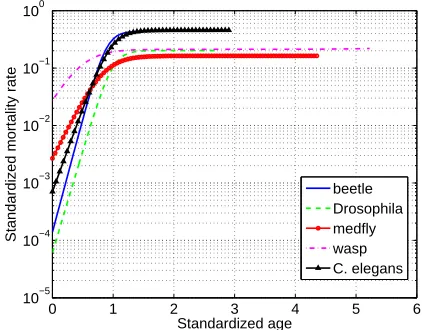
5.5 Some animal mortality patterns
In an exploration of the effects of heterogeneity on the distribution of age at death, Hori-uchi (2003) estimated G-G parameters from data on laboratory populations of five species of invertebrate animals: a bean beetle (Callosobruchus maculatus), the medfly (Ceratitis capitata), the fruit flyDrosophila melanogaster, the nematodeCaenorhabditis elegans, and a parasitoid wasp (Diachasimimorpha longicaudata.) Because the estimated G-G parameters for these species do not appear in the original paper, they are listed here in Table B.1.
mortality rates reach a plateau at an age of about 1 life expectancy, at a standardized mortality rate of 0.1 to 0.5. Further interspecific analyses would be interesting.
Figure 10: The marginal mortality rateµ∗(t)as a function of standardized aget, for five species of invertebrate animals, based on G-G parameters estimated by Horiuchi (2003). The age abcissa is scaled by dividing age by the life expectancy at birth. The mortality rate is standardized by multiplying by the same life expectancy
0 1 2 3 4 5 6
10−5 10−4 10−3 10−2 10−1 100
Standardized age
Standardized mortality rate
beetle Drosophila medfly wasp C. elegans
6. Heterogeneous frailty vs. individual stochasticity: partitioning
variance in longevity
Inter-individual variance in longevity is often taken to be evidence of heterogeneity or inequality among individuals in their mortality risks. However, variance also arises from
individual stochasticity, the random variation to which the fates of indivduals are subject even if they experience exactly the same risks at every stage of the life cycle (Caswell 2009, 2011; Tuljapurkar, Steiner, and Orzack 2009). The only way to evaluate the contri-bution of heterogeneity is to partition the variance into components due to heterogeneity and to individual stochasticity. Frailty models permit us to do so.
Figure 11: The variance of longevity, at ages 0 and 60, as a function of the variance of the initial frailty distribution. (a) The
gamma-Gompertz model, calculated from parameters reported by Missov (2013) for Swedish females in 1950. (b) The
gamma-Makeham model, calculated from parameters reported by Zarulli et al. (2013) for a cohort model of the female population of Turin. (b) The gamma-Siler model, calculated from parameters reported by Engelman, Canudas-Romo, and Agree (2013) for Swedish females born in 1900. The vertical lines indicates the observed values of initial variance in frailty
(a) Gamma-Gompertz model
10−4 10−2 100 102
0 200 400 600 800 1000 1200
Gamma variance
Variance of longevity
0 60
(b) Gamma-Makeham model
10−4 10−2 100 102
0 200 400 600 800 1000 1200
Gamma variance
Variance of longevity
0 60
(c) Gamma-Siler model
10−4 10−2 100 102
0 500 1000 1500 2000 2500
Gamma variance
Variance of longevity
This is not always the case. Table 2 compares the decomposition of the variance for Swedish females (using the G-G, gamma-Makeham, and gamma-Siler mdoels) with that for the animal species from Horiuchi (2003). In the human populations, heterogeneity accounts for only 2–7% of the variance in longevity. In the experimental animal data, heterogeneity accounts for 46% to 83% of the variance in longevity. These patterns de-serve further empirical investigation.
Table 2: Decomposition of the variance in longevity for human populations and laboratory populations of invertebrate species. The varianceσ2 in initial frailty, the varianceV(η)in longevity and the components ofV(η)due to individual stochasticity and to heterogeneous frailty, and the proportion of the variance due to heterogeneity. Species are listed in order of increasing initial variance in frailty. Data from Horiuchi (2003)
Species σ2 V(η) Stochasticity Heterogeneity Proportion
Sweden 1950 G-G 0.122 122.9 114.1 8.72 0.071
Turin G-M 0.096 351.6 347.3 104.3 0.012
Sweden 1900 G-S 0.120 1091.7 1074.1 17.60 0.016
nematode 0.90 18.0 9.7 8.3 0.46
fruit fly 0.94 88.1 46.1 42.0 0.48
beetle 1.31 12.7 5.2 7.5 0.59
medfly 1.34 81.8 29.5 52.3 0.64
wasp 2.18 30.3 5.1 25.2 0.83
7. Conclusions
the marginal age-specific mortality and survival functions, and a complete set of statistics of longevity.
Table 3 gives a step-by-step protocol for the analysis of the G-G and other frailty models. Other choices of baseline mortality rate (e.g., the Makeham model or the Siler model considered in Section 5.1), the action of frailty (e.g., accelerated failure time mod-els), the dynamics of frailty (e.g., the frailty diffusion models discussed in Section 5.4), or the initial distribution of frailty require only simple modifications of the appropriate steps in Table 3.
Table 3: A protocol for analysis of the gamma-Gompertz model
1. Specify the Gompertz parameters aand b, and the gamma distribution paramater k. Choose values for the numbers of age classes ω and the number of frailty classesg.
2. Generate the baseline mortality vectorµ0from (10)
3. Specify the frailty classeszi,i= 1, . . . , g, and the discrete approximation to the gamma distributionπ. Logarithmically-spaced frailty classes are recommended.
4. Create the matricesUi, fori= 1, . . . , g, as in equation (12). 5. Create the block diagonal matricesUandDaccording to (13).
6. Create the joint transition matrixU˜ according to (18). 7. Analyze the model
(a) Compute the fundamental matrixN˜ from (20). (b) Compute the marginal survival functions∗from (22). (c) Generate the marginal fundamental matrixN∗from (24).
(d) Generate life expectancy and other indices of longevity from N∗
using (25)–(36).
8. Project the dynamics of the age-frailty distributionn˜(t)with (41). Obtain the marginal age abundance vector n∗ using (43) and the marginal age distribution vectorp∗using (44).
9. Obtain the marginal frailty abundance vectorm∗using (45) and the frailty distributionπ(t)from equation (46).
10. If desired, create the mortality matrixM˜ and generate the distributions of age and of frailty at death from equations (38)–(40).
7.1 Some pleasant properties of the matrix formulation
tempta-tion to be resisted. Although the matrix formulatempta-tion of frailty models has many pleasant properties, it complements, rather than replaces, other formulations (e.g., matrix notation is unlikely to lead to easily interpretable symbolic results). Some properties worth noting include the following.
1. Easy computation: all the statistics of longevity, and all the dynamics of the joint age-frailty distribution, are readily computed. A MATLAB script to compute the results for the Swedish example from Missov (2013) is included in the Supplemen-tary Material to this paper.
2. Variance decomposition: because the matrix formulation clearly separates the het-erogeneity from the stochastic process of mortality, it facilitates decomposition of the variance in longevity into their contributions.
3. Generality: the analysis extends to any age×frailty model (Table 3) and, indeed, to stage-classified (e.g., educational status, health status) or multi-stage models as well as age-classified models.
4. Population growth and stable population theory: the matrix formulation has the potential to incorporate heterogeneous frailty into models of population growth, and hence into stable population theory (Caswell 2012).
5. Sensitivity analysis: because the results are obtained by matrix operations, they are directly amenable to sensitivity analysis using matrix calculus methods (e.g., Caswell 2006, 2007, 2008, 2009, 2012, 2013; van Raalte and Caswell 2013; Engel-man, Caswell, and Agree 2014) Such methods will provide the levels of sensitivity of the moments of longevity, the joint distribution of age and stage at death, and the survivorship and mortality functions to changes in any of the parameters of the model. Results will be presented elsewhere.
6. Likelihood and parameter estimation. The formulation as an absorbing Markov chain may potentially contribute to the computation of likelihood functions from data on individuals. Such approaches have been used by animal ecologists ana-lyzing mark-recapture data (e.g., Caswell and Fujiwara 2004) and implemented in some software packages (Pradel 2005; Choquet and Nogue 2010). Because frailty is inherently unobserved, issues of identifiability arise, which can also sometimes be addressed using the Markov chain formulation (Hunter and Caswell 2009).
8. Acknowledgments
References
Abramowitz, M. and Stegun, I.A. (1965). Handbook of mathematical functions. Dover.
Anderson, J.E. and Louis, T.A. (1995). Survival analysis using a scale change random effects model. Journal of the American Statistical Association 90(430): 669–679.
doi:10.2307/2291080.
Caswell, H. (2001). Matrix population models: construction, analysis, and interpreta-tion. Sunderland, MA: Sinauer Associates.
Caswell, H. (2006). Applications of markov chains in demography. In: Langville, A.N. and Stewart, W. (eds.).MAM2006: Markov Anniversary Meeting. Boson Books: 319– 334.
Caswell, H. (2007). Sensitivity analysis of transient population dynamics. Ecology Let-ters10(1): 1–15.doi:10.1111/j.1461-0248.2006.01001.x.
Caswell, H. (2008). Perturbation analysis of nonlinear matrix population models. Demo-graphic Research18(3): 59–116.doi:10.4054/DemRes.2008.18.3.
Caswell, H. (2009). Stage, age and individual stochasticity in demography. Oikos
118(12): 1763–1782.doi:10.1111/j.1600-0706.2009.17620.x.
Caswell, H. (2011). BeyondR0: Demographic Models for Variability of Lifetime Repro-ductive Output. PloS ONE6(6): e20809.doi:10.1371/journal.pone.0020809.
Caswell, H. (2012). Matrix models and sensitivity analysis of populations classified by age and stage: a vec-permutation matrix approach.Theoretical Ecology5(3): 403–417.
doi:10.1007/s12080-011-0132-2.
Caswell, H. (2013). Sensitivity analysis of discrete Markov chains via matrix
cal-culus. Linear Algebra and its Applications 438(4): 1727–1745. doi:10.1016/
j.laa.2011.07.046; 16th ILAS Conference Proceedings, Pisa 2010.
Caswell, H. and Fujiwara, M. (2004). Beyond survival estimation: mark-recapture, ma-trix population models, and population dynamics.Animal Biodiversity and Conserva-tion27(1): 471–488.
Caswell, H. and Salguero-G´omez, R. (2013). Age, stage and senescence in plants. Jour-nal of Ecology101(3): 585–595.doi:10.1111/1365-2745.12088.
Cha, J.H. and Finkelstein, M. (2013). The failure rate dynamics in heterogeneous pop-ulations. Reliability Engineering and System Safety 112: 120–128. doi:10.1016/ j.ress.2012.11.012.
Fonc-tionnelle et Evolutive.
Engelman, M., Canudas-Romo, V., and Agree, E.M. (2013). Frailty in transition: vari-ation and vulnerability in aging populvari-ations. Center for Demography and Ecology, University of Wisconsin-Madison.
Engelman, M., Caswell, H., and Agree, E.M. (2014). Why do lifespan variability
trends for the young and old diverge? Demographic Research30(48): 1367–1396.
doi:10.4054/DemRes.2014.30.48.
Feichtinger, G. (1971). Stochastische Modelle demographischer Prozesse. Berlin: Springer-Verlag.
Gage, T.B. (1998). The comparative demography of primates: with some comments on the evolution of life histories. Annual Review of Anthropology 27: 197–221.
doi:10.1146/annurev.anthro.27.1.197.
Gavrilov, L.A. and Gavrilova, N.S. (1992). The biology of life span: A quantitative approach. New York: Harwood Academic Publishers.
Henderson, H.V. and Searle, S.R. (1981). The vec-permutation matrix, the vec operator and kronecker products: A review. Linear and Multilinear Algebra9(4): 271–288.
doi:10.1080/03081088108817379.
Horiuchi, S. (2003). Interspecies Differences in the Life Span Distribution: Humans versus Invertebrates.Population and Development Review29: 127–151.
Hunter, C.M. and Caswell, H. (2005). The use of the vec-permutation matrix in spa-tial matrix population models. Ecological Modelling188(1): 15–21. doi:10.1016/ j.ecolmodel.2005.05.002.
Hunter, C.M. and Caswell, H. (2009). Rank and Redundancy of Multistate
Mark-Recapture Models for Seabird Populations with Unobservable States. In: Thomp-son, D.L., Cooch, E.G., and Conroy, M.J. (eds.).Modeling Demographic Processes In Marked Populations. New York: Springer: 797–825. doi:10.1007/978-0-387-78151-8 37.
Iosifescu, M. (1980).Finite markov processes and their applications. New York: Wiley.
Keiding, N., Andersen, P.K., and Klein, J.P. (1997). The role of frailty models and ac-celerated failure time models in describing heterogeneity due to omitted covariates.
Statistics in Medicine16(2): 215–224.
Keyfitz, N. and Caswell, H. (2005). Applied mathematical demography. New York: Springer.
by a multivariate normal regression model. Biometrics55(2): 497–506.
Kondor, R.I. and Lafferty, J.D. (2002). Diffusion Kernels on Graphs and Other Discrete Input Spaces. In: Sammut, C. and Hoffmann, A.G. (eds.). Proceedings of the 19th International Conference on Machine Learning (ICML 2002). Morgan-Kaufman Pub-lishers: 315–322.
Le Bras, H. (1976). Lois de mortalit´e et ˆage limite.Population31(3): 655–692.
Magnus, J.R. and Neudecker, H. (1979). The commutation matrix: some properties and applications.Annals of Statistics7(2): 381–394.
Missov, T.I. (2013). Gamma-Gompertz life expectancy at birth. Demographic Research
28(9): 259–270. doi:10.4054/DemRes.2013.28.9.
Missov, T.I. and Finkelstein, M. (2011). Admissible mixing distributions for a general class of mixture survival models with known asymptotics. Theoretical Population Bi-ology80(1): 64–70.doi:10.1016/j.tpb.2011.05.001.
Pan, W. (2001). Using frailties in the accelerated failure time model. Lifetime Data Analysis7(1): 55–64.doi:10.1023/A:1009625210191.
Pradel, R. (2005). Multievent: An Extension of Multistate Capture–Recapture Models to Uncertain States.Biometrics61(2): 442–447.
Tuljapurkar, S., Steiner, U.K., and Orzack, S.H. (2009). Dynamic heterogeneity in life histories. Ecology Letters12(1): 93–106.doi:10.1111/j.1461-0248.2008.01262.x.
van Raalte, A.A. and Caswell, H. (2013). Perturbation analysis of indices of lifespan variability.Demography50(5): 1615–1640.doi:10.1007/s13524-013-0223-3.
Vaupel, J.W. (2010). Biodemography of human ageing. Nature 464: 536–542.
doi:10.1038/nature08984.
Vaupel, J.W. and Carey, J.R. (1993). Compositional interpretations of medfly mortality.
Science260(5114): 1666–1667.
Vaupel, J.W., Carey, J.R., Christensen, K., Johnson, T.E., Yashin, A.I., Holm, N.V.,
Iachine, I.A., Kannisto, V., Khazaeli, A.A., and Liedo, P. (1998).
Biodemo-graphic Trajectories of Longevity. Science 280(5365): 855–860. doi:10.1126/
science.280.5365.855.
Vaupel, J.W., Manton, K.G., and Stallard, E. (1979). The impact of heterogeneity in indi-vidual frailty on the dynamics of mortality.Demography16(3): 439–454.doi:10.2307/ 2061224.
Vaupel, J.W. and Yashin, A.I. (1985). Heterogeneity’s ruses: some surprising effects of selection on population dynamics.American Statistician39(3): 176–185.doi:10.2307/ 2683925.
Vaupel, J.W. and Yashin, A.I. (2006). Unobserved population heterogeneity. In: De-mography: Analysis and Synthesis: A Treatise in Population Studies. Academic Press: 271–278, vol. 1.
Vaupel, J.W., Yashin, A.I., and Manton, K.G. (1988). Debilitation’s aftermath: Stochas-tic process models of mortality. Mathematical Population Studies 1(1): 21–48.
doi:10.1080/08898488809525259.
Wienke, A. (2010). Frailty models in survival analysis. Boca Raton, Florida: Chapman & Hall/CRC.
Yashin, A.I., Iachine, I.A., and Begun, A.S. (2000). Mortality modeling: A review.
Mathematical Population Studies8(4): 305–332.doi:10.1080/08898480009525489.
Yashin, A.I., Vaupel, J.W., and Iachine, I.A. (1994). A duality in aging: the equivalence of mortality models based on radically different concepts. Mechanisms of Ageing and Development74(1–2): 1–14.doi:10.1016/0047-6374(94)90094-9.
Appendix A: Gamma-Makeham and Gamma-Siler models
This appendix collects results on the statistics of longevity and the dynamics of frailty for the gamma-Makeham model and the gamma-Siler model, in the same format used for results from the G-G model in Figures 2 and 3.
A.1 Gamma-Makeham
Figure A.1: Statistics of longevity for the gamma-Makeham model, as a function of age. Calculated from parameters reported by Zarulli et al. (2013) for a cohort model for the female population of Turin
(a) Life expectancy
0 20 40 60 80 100 120
0 10 20 30 40 50 60 70 80 90
Age
Life expectancy
(b) Standard deviation of longevity
0 20 40 60 80 100 120
0 5 10 15 20
Age
SD of longevity
(c) CV of longevity
0 20 40 60 80 100 120
0.2 0.3 0.4 0.5 0.6 0.7 0.8 0.9
Age
CV of longevity
(d) Skewness of longevity
0 20 40 60 80 100 120
−2.5 −2 −1.5 −1 −0.5 0 0.5 1 1.5 2
Age
Figure A.2: Statistics of frailty, and marginal mortality rateµ∗, for the gamma-Makeham model, as a function of age. Calculated from parameters reported by Zarulli et al. (2013) for a cohort model for the female population of Turin
(a) Mean frailty
0 20 40 60 80 100 120
0.4 0.5 0.6 0.7 0.8 0.9 1
Age
Mean frailty
(b) Standard deviation of frailty
0 20 40 60 80 100 120
0.1 0.15 0.2 0.25 0.3 0.35
Age
SD frailty
(c) Marginal mortality
0 50 100 150
10−3 10−2 10−1 100 101
Age
A.2 Gamma-Siler
Figure A.3: Statistics of longevity for the gamma-Siler model, as a function of age. Calculated from parameters reported by Engelman,
Canudas-Romo, and Agree (2013) for Swedish females born in 1900
(a) Life expectancy
0 20 40 60 80 100 120
0 10 20 30 40 50 60 70 80
Age
Life expectancy
(b) Standard deviation of longevity
0 20 40 60 80 100 120
0 5 10 15 20 25 30 35
Age
SD of longevity
(c) CV of longevity
0 20 40 60 80 100 120
0.35 0.4 0.45 0.5 0.55 0.6 0.65 0.7 0.75
Age
CV of longevity
(d) Skewness of longevity
0 20 40 60 80 100 120
−1.5 −1 −0.5 0 0.5 1 1.5 2 2.5
Age
Figure A.4: Statistics of frailty, and marginal mortality rateµ∗, for the gamma-Siler model, as a function of age. Calculated from parameters reported by Engelman, Canudas-Romo, and Agree (2013) for Swedish females born in 1900
(a) Mean frailty
0 20 40 60 80 100 120
0.1 0.2 0.3 0.4 0.5 0.6 0.7 0.8 0.9 1
Age
Mean frailty
(b) Standard deviation of frailty
0 20 40 60 80 100 120
0.05 0.1 0.15 0.2 0.25 0.3 0.35 0.4
Age
SD frailty
(c) Marginal mortality
0 50 100 150
10−3 10−2 10−1 100
Age
Appendix B: Parameters for animal species
Table B.1: Gamma-Gompertz parameters for the invertebrate animal species analyzed by Horiuchi (2003); data provided by Horiuchi (personal communication)
Species a b k
Medfly 0.0027 0.2168 0.7530
Nematode 6.9970×10⁻⁴ 0.4059 1.1264
Wasp 0.0278 0.4575 0.4640
Drosophila 6.0558×10⁻⁵ 0.1878 1.0796