Bloom Filters for Filesystem Forensics

University of New Orleans University of New Orleans

ScholarWorks@UNO

ScholarWorks@UNO

University of New Orleans Theses and

Dissertations Dissertations and Theses

12-15-2006

Bloom Filters for Filesystem Forensics

Bloom Filters for Filesystem Forensics

Rachel Bourg

University of New Orleans

Follow this and additional works at: https://scholarworks.uno.edu/td

Recommended Citation Recommended Citation

Bourg, Rachel, "Bloom Filters for Filesystem Forensics" (2006). University of New Orleans Theses and Dissertations. 1288.

https://scholarworks.uno.edu/td/1288

This Thesis is protected by copyright and/or related rights. It has been brought to you by ScholarWorks@UNO with permission from the rights-holder(s). You are free to use this Thesis in any way that is permitted by the copyright and related rights legislation that applies to your use. For other uses you need to obtain permission from the rights-holder(s) directly, unless additional rights are indicated by a Creative Commons license in the record and/or on the work itself.

Bloom Filters for Filesystem Forensics

A Thesis

Submitted to the Graduate Faculty of the

University of New Orleans In partial

fulfillment of the Requirements for the

degree of

Masters of Science In

Computer Science

Information Assurance

By

Rachel Bourg

B.S. University of New Orleans, 2002

Dedication

Acknowledgements

To my late grandfather, thank you for the foundation you gave me as a child, without which any of this would have been possible. To Dr. Vassil Roussev, thank you for the idea for my thesis, but mainly your patience, guidance, and your many revisions of my paper.

Also, thank you to my Thesis committee. To my stepson, Christopher, I hope all my hard work on this paper is an example to you. And last but not least to my wife, thank you for all your support, your patience with me as I spent time working on my project, and all your encouragement to help me become a better person. But most of all, I thank you for all the love you give to me every day. I love you, Deana, with all my heart.

Table of Contents

List of Figures...v

Abstract... vi

Chapter 1: Introduction...1

Chapter 2: Related Work ...4

2.1 Bloom Filters ...4

2.1.1 Basic Bloom Filters...4

2.1.2 Hierarchical Bloom Filters...8

2.1.3 Counting Bloom Filters...8

2.1.4 Compressed Bloom Filters...9

2.2 Tools for Correlation...9

2.2.1 sif...9

2.2.2 Hard Drive Correlation ...10

2.2.3 md5deep ...10

2.2.4 ssdeep...11 Chapter 3: Tool Design and Implementation...12

3.1 Scenarios...12

3.1.1 Collaborative Investigations ...12

3.1.2 Known File Identification...13

3.1.3 Multiple Target Correlation ...14

3.2 Design ...14

3.2.1 Single User Mode ...16

3.2.2 Single User / Separate Client and Server...16

3.2.3 Multiple User / Single Server ...17

3.2.4 Multiple Servers...18

3.2.5 Filter Comparison ...19

3.3 Implementation Details...20

3.4 Command Line Options...21

3.4.1 Filter Generation Options ...21

3.4.2 Client Options ...25

3.4.3 Query Options...26

3.4.4 Comparison Options ...27 Chapter 4: Experimental Evaluation...28

4.1 Verification ...28

4.1.1 False Positive Verification...29

4.1.2 Matching Bit Probability Verification ...30

4.2 Performance Results ...30

4.3 Similarity Experiments ...34

4.3.1 Similarity of /usr/bin on KNOPPIX Versions ...35

4.3.2 Similarity of the Standard C Library (libc) on KNOPPIX Versions ...38 Chapter 5: Conclusion...41

5.1 Summary...41

5.2 Future Work...42

References...44

List of Figures

Equation 2.1: Probability that a specific bit is 0 ...5

Equation 2.2: False positive probability ...5

Equation 2.3: Probability that a specific bit in two filters is 1...6

Equation 2.4: Probability that given C bits in common if the rest are 0...6

Equation 2.5: Probability that C bits are in common between two filters ...7

Equation 2.6: Normal distribution parameters...7

Figure 2.7: Example probability density functions...7

Figure 3.1: Merged Front-end and Back-end...16

Figure 3.2: Single User / Separate Client and Server ...17

Figure 3.3: Multiple User / Single Server...18

Figure 3.4: Multiple Servers ...19

Figure 3.5: Filter Comparison...20

Equation 4.1: False Positive Rate ...29

Figure 4.2: Example False Positive Rates...30

Figure 4.3: md5bloom vs. md5deep performance comparison ...33

Figure 4.4: KNOPPIX /usr/bin comparison / r = 8 ...36

Figure 4.5: KNOPPIX /usr/bin comparison / r = 4 ...37

Figure 4.6: KNOPPIX /usr/bin comparison / r = 2 ...37

Figure 4.7: KNOPPIX /usr/bin comparison p-values / r = 2 ...38

Figure 4.8: KNOPPIX libc comparison / r = 8 ...39

Figure 4.9: KNOPPIX libc comparison / r = 4 ...40

Abstract

Digital forensics investigations become more time consuming as the amount of data to be

Chapter 1: Introduction

Digital forensics is the investigation of computers and other digital media for either court cases or internal corporate investigations. Although forensic investigations can be done on any digital data, large file systems on hard drives are the most common forms of digital evidence. Many

investigations involve correlating many large file systems, which considerably increases the amount of effort required to perform the investigations. Hard drive capacities are continually growing, so the amount of data that will need to be potentially investigated continues to grow. There is a

growing performance gap between hard drive capacity and hard drive bandwidth and latency, and this will continue to grow; over the last 20 years, bandwidth has increased 100 times, latency has

decreased by 10 percent, but capacity has increased by over 2400 times [10]. The forensic tools being used today are time consuming and make investigations of large amounts of data very cumbersome. For this reason, there are considerable backlogs in digital forensics labs and will continue to be for the foreseeable future. Automated tools can be used, but they could possibly miss some important evidence. More efficient interactive tools could make manual investigations more focused to identify important evidence quicker. This work aims to alleviate this problem by making investigations of large amounts of data more efficient and more interactive by creating more effective tools for digital forensics investigators. The tool we developed can be used on data recovered from devices such as cell phones, personal digital assistants (PDAs), USB keys, and digital cameras, but they do not present a scalability problem that large hard drives do.

identify that specific data at a later time. These numbers, or message digests, can be used as

―fingerprints‖ to classify files as either important or irrelevant using lists of hashes of known files.

Data can be fed through the function and the resulting message digest compared with the original digest. If they match, then the messages are assumed to be identical. Hash functions are also used to determine evidence integrity by hashing an entire hard drive image before and after an investigation. As long as the two hashes match, the evidence has not been modified.

A cryptographic hash function is a collision-resistant hash function which means that it is

computationally infeasible to find a message that matches a given result, other than the one used to generate the result, or to find two messages that have an identical result. Cryptographic hash functions, such as MD5 or SHA-1, are used by current utilities to identify known files. By design, when even a single bit change is made to a known file, a radically different message digest is returned by the hash function. This problem is encountered often due to the dynamic nature of many

operating systems and software installations. The updates of these files cause the lists of known file hashes to age quickly. Therefore, there needs to be a way to test for similarity as files can be

dynamically updated often by automatic update utilities.

processing this data. Virtual memory would not help due to random nature of hash table

accesses, which would be painfully slow on secondary storage. So there needs to be a way to compress these hashes to be able to fit in main memory for efficient searches.

Bloom filters are space-efficient data structures used to test for set membership. The design of Bloom filters save space, but also gives the possibility of false positives. By modifying attributes of the Bloom filter the probability of false positives can be quantified and, therefore, configured to meet the requirements of the application. For the example above, it is possible to store the 16 GB of hashes in 2 GB of RAM with a false positive rate of less than 1 percent.

The benefits that Bloom filters provide are not limited to more efficient representation. Directly comparing (the binary representation of) filters provide a means to statistically determine how closely related two filters, or the data that they were created from, are. We show that comparing Bloom filters is very useful for determining similarity of various types of data, no matter what the source of the data is. For example, we compare versions of libraries and binary files in different versions of Linux distributions. The observed similarity of the Bloom filters generated from these different distributions correlate the versions well, and even shows a linear similarity relationship between consecutive versions.

Chapter 2: Related Work

Much work has been done with Bloom filters since they were introduced in 1970 in Burton H. Bloom’s paper ―Space/Time Trade-offs in Hash Coding with Allowable Errors [2].‖ They have

been used in a variety of areas, but mainly network applications. There have been many extensions to the initial data structure proposed by Bloom. Here we give a short summary of the different types of Bloom filters that have been proposed. The purpose of this chapter is to provide a brief overview of Bloom filters and their different types, and generally follows the extensive discussion in [3]. Also, to the best of our knowledge, no use of direct comparison of Bloom filters has been published.

Recently, there also has been some work on forensic data correlation. Here we summarize some tools that have been developed, and show some of their uses. The tools we describe have their uses, but most of them are text-based, and either does not support binary files at all or do not handle them well.

2.1 Bloom Filters

2.1.1 Basic Bloom Filters

k hash functions and test the corresponding bits. If any of those bits are zero, then the item is not

contained in the filter; therefore there are no false negatives. However, there is a possibility that some or all the bits were set by other items’ hash values, which could result in false positives. However, through careful selection of m, k, and m/n, the ratio of bits per element in the filter, the probability of getting a false positive can be quantified.

Once all elements are added to the filter, the probability that a specific bit is 0, given that the hash functions are perfectly and uniformly random is defined by the following function:

kn⎛ 1 ⎞− kn / m

p =⎜1 −⎟≈ e ⎝m

⎠

Equation 2.1: Probability that a specific bit is 0

A false positive occurs when all the k tested bits are not 0. For the purposes of this discussion, it is safe to assume that all the bits in a Bloom filter B are independently left zero with probability p, and set to one with a probability of 1 – p. (We provide a verification of this formula in section 4.1.1.) From this, probability of a false positive can be expressed as:

⎛⎞k ⎜⎛₋ 1

⎞ kn

⎟−kn / mk k

P_fp = 1 −⎜1 ⎟≈ (1 − _⎜⎟ e ) = (1− p) ⎝ m ⎠

⎝⎠

Equation 2.2: False positive probability

Another use of Bloom filters is to determine similarity of data sets. This can be done by

comparing two filters directly. This can show similarity of two data sets without actually querying the filter with hashes. For the comparison to be possible, each filter must have the same size. We define a matching bit to be a bit set to 1 in 2 filters in the same place. The more bits matching between the two filters, the more likely the data sets that generated the filters come from similar data. However, the probabilistic nature of Bloom filters that cause false positives can also cause bits to match between two filters generated from totally random data.

In this case, we need a way to measure whether the amount of bits matching indicates similarity or just random matches. Using Equation 2.1, the probability of a bit being set to 1, is 1–p. So for two Bloom filters B1 and B2, the probability of a bit being set to 1 in each filter is as follows:

1

p = 1 − ⎛⎜1 − 1

⎟⎞

kn

≈ 1 − e −kn1/ m

1

⎝

m ⎠

kn₁ ⎛ 1 ⎞−kn1/ m

p = 1 −⎜1 −⎟≈ 1 − e

2

⎝m

⎠

Equation 2.3: Probability that a specific bit in two filters is 1

From this, we get the fact that the probability that specific C bits are in common between each filter is p1

C p2

C

p-(C) where p-(C) is the probability that the remaining m – C bits are zero. Taking into account all ways that bits can be selected, p-(C) can be calculated as follows:

m−C

⎧⎛ ⎪ i _⎞

ii m−C −i ⎪

⎫ p₋ (C_{) = ∑}⎨

⎜⎜ (1− p1) (1− p₂) [ p₁(1− p₂) + p₂ (1− p₁)] ⎬ i=0

⎩⎪⎝ m − C

⎠ _⎭⎪

Equation 2.4: Probability that given C bits in common if the rest is 0

Consequently, the probability that C bits are in common between two filters is: ⎛C ⎞

p(C) = _{( pp )}C p (C)

12 −

Equation 2.5: Probability that C bits are in common between two filters

This allows us to calculate the probability that a specific amount of matching bits C occurred by chance.

If the probability is very small for a specific C, it is likely that the two filters were generated from similar data. Calculating p(C) is very cumbersome, but given the main terms of the function, a normal distribution approximation can be found by assuming that the hash functions (subhashes) are independent. In practice, such an assumption is quite reasonable for cryptographic hashes. Using standard statistical averaging, it can be shown that under the assumption of independence, the parameters of the normal distribution are: mean = m * p₁* p₂

std.dev. =

m * p * p * (1− p * p ) 12 12

Equation 2.6: Normal distribution parameters

See figure 1 for some example distribution curves.

One extension to Bloom’s design is Hierarchical Bloom Filters (HBF), which can be used to

determine the location of data in a large amount of data, rather than just the existence of the data in the large amount of data [11]. HBFs are basically collections of Block-Based Bloom Filters (BBFs). BBFs are created by hashing a set of data with a given block size, block by block. But before each block is hashed, its offset in the data set is appended to the block data to be hashed along with the data. The collection of BBFs is organized by levels, with the block size doubling as the levels increase. If two blocks of data are found in the filter at level 0, or the filter with the smallest block size, then you can assume, taking into account the false positive rate, that both blocks of data are located in the filter. However, if these two blocks are concatenated together and hashed, then the filter at level 1 can be queried with this hash. If this hash is found, then you can assume that, again taking into account the false positive rate, these two blocks occurred consecutively in the filter. Otherwise, the blocks occurred in completely different locations in the data set.

2.1.3 Counting Bloom Filters

One limitation of Bloom filters that makes it not useful for changing sets is that deletion is not

possible, since false negatives are not allowed. If deletion were allowed, the way it could possibly be implemented is to set all the bits that the k hash functions indicate to 0. However, if there is any overlap, that is if any hashes were inserted and one of the locations it had to set were already one, a false negative would occur because the item that had previously set the bit to 1 would now not be detected in the filter. One way solve this problem is to use Counting Bloom Filters (CBFs). The difference between regular Bloom filters and CBFs is that instead of a single bit for each offset in the filter, there are multiple bits for each offset in the filter. With CBFs, insertion is done by

done by decrementing the k locations. Lookups are done by checking if the k locations are not

equal to 0 [3].

2.1.4 Compressed Bloom Filters

In network applications, it may be necessary to send Bloom filters between nodes. Mitzenmacher raises the question if something can be gained by compressing a Bloom filter [8]. Taking the optimization from standard Bloom filters where p = 1/2. This means that each bit in the Bloom filter has an equal probability to be either 0 or 1. Assuming good random hash functions, the Bloom filter is basically a random string of 0’s and 1’s, which does not compress very well. He proposes to

choose a k to where each bit in the filter is 1 with a probability of 1/3. This allows the filter to be compressed before transmission and decompressed at the other end to be used by the application.

2.2 Tools for Correlation

2.2.1

sif

The utility sif is mainly used to detect similarity of text files, by using a method called ―Approximate Fingerprinting.‖ [7] This involves selecting a random set of ―anchors‖, and these anchors are

searched for in the files to be compared. When these anchors are found in a file, the checksum of a fixed number of characters previous to this anchor in each file is calculated. Each of these

checksums, along with their associated anchors, is saved for each file as their ―fingerprints.‖ To

2.2.2 Hard Drive Correlation

To correlate hard drives, Garfinkel [4] uses pseudo-unique identifying information such as email addresses, credit card numbers, and social security numbers. The idea is that these pieces of data are unique enough that if they were to occur on more than one evidence item, then these hard drives could be considered related. This idea is very useful, as it could detect such things as stolen credit card numbers or relating two separate hard drives to determine that the owners of them were communicating, and possibly involved in criminal activity together. However, this is strictly text-based and would not be able to detect similar binary files between two hard drives. However, text searching in large targets requires much random I/O, since hard drive data cannot fit in memory. Text searching also tends to be computationally expensive. This method may be very useful, but since it tends to be slow, it is not as efficient as the tools we developed.

2.2.3

md5deep

2.2.4

ssdeep

ssdeep is a utility described in [5], which uses context-triggered piecewise hashing to create

Chapter 3: Tool Design and Implementation

To solve the problem presented in Chapter 1, we have developed a utility called md5bloom. This utility is an implementation of Bloom filters, with client/server functionality. There are options to generate filters from MD5 hashes derived from many different sources, such as hashes generated from a data stream or hexadecimal text representations of MD5 hashes. It also provides a TCP/IP server for query submission. In addition to the TCP/IP server, the utility can also perform queries on the filter with hashes derived from the same data sources as the generation options, but without a separate server. The TCP/IP server allows query servers to be advertised for many different clients to send requests to them from anywhere on the Internet, whereas the options to query without a separate server is better suited for one user that needs to send many queries to a filter quickly.

3.1 Scenarios

There are several investigative scenarios in which our tool can be used. There are lab situations where a filter could be used simultaneously for investigators collaboratively working on a single investigation or as a common filter for multiple investigations. There is also the possibility of creating a high-end dedicated filter server that could advertise many filters that have been generated from previous investigations for an investigator to correlate them with existing investigations. Filters could also be used by a single user, with a client and server merged into the same address space to eliminate any network overhead.

3.1.1 Collaborative Investigations

simultaneously. This would prevent hold ups due to another investigator using a piece of

evidence that is needed to follow a lead discovered from another piece of evidence. The drive could be retrieved from the evidence locker and reimaged, but that would waste time. It could be

conceivable to have enough shared space to store images of evidence for all users to access, but instead of storing all the data on a shared drive, Bloom filters could be stored on a shared drive. This would allow investigators to quickly correlate data from two pieces of evidence without having the actual data. If something relevant is detected in the Bloom filter, then the actual data can be

retrieved. Also, to conserve computing power on a workstation, a Bloom filter server can be run on a high end server to listen for queries. This would also prevent inadvertent modification of shared Bloom filters.

3.1.2 Known File Identification

3.1.3 Multiple Target Correlation

One area of digital forensics investigations that is becoming increasingly important is to correlate many different pieces of evidence. Since portable digital devices, cell phones, PDAs, USB keys, etc. have become ubiquitous, it is necessary to be able to associate the data from these devices to other pieces of evidence. Also, multiple PCs in a household, or even per user, are common, so there needs to be a way to correlate data between these devices. Also, for investigative leads, it may be useful to correlate evidence from previous cases, to associate the data, thereby associating the users, to

possibly identify people involved in similar criminal activities. Using our tool, performing this correlation can be very efficient. Comparing Bloom filters generated from two sets of data to be correlated gives a statistical analysis to identify the similarity the two sets of data as well as the confidence that the similarity that was detected occurred by chance. Bloom filters from previous cases can be loaded as server to be queried at any time by investigators, to aid in the correlation process. For future work (section 5.1.2), there will also be a specialized front-end to allow

correlation of data to multiple Bloom filter servers simultaneously. We also will provide a means to correlate multiple targets at once, as well as providing statistical analysis of the comparisons done.

3.2 Design

components for filter creation, loading from disk, and a server for querying filters and searching

filters. The front-ends either send hash queries or hash insertion requests to servers to perform the appropriate option on the filter used by the server.

We chose to make the back-ends multithreaded due to the fact that filter lookups are easily

parallelized. Also, the front-ends tend to send many queries at once, so a multithreaded back-end increases efficiency considerably. The back-end is also multithreaded to be able to handle many clients simultaneously. Also to prevent the front-ends from having to wait for responses before reading more data to calculate hashes for queries, we also made the front-ends multithreaded. This also allows the front-end to do file I/O while receiving responses from the network at the same time. This also allows full utilization of dual-core processors by both the front and back-ends to

maximize the use of the computing power of the system.

3.2.1 Single user mode

In cases where a filter is relevant only to a particular case, and if there is only one user needing to query it at a time, the front-end and back-end can be merged, where the queries can be performed by only memory accesses, instead of via the network. This way, network overhead is avoided, which speeds up responses considerably. In this scenario, the Bloom filter is read in from a file and loaded into memory. At this point, it is ready for requests from the front-end. Then, the query data is read in, hashes are calculated from this data, and then these hashes are sent to the back-end as queries. As the back-end receives these queries, they are checked against the loaded filter, and then a response is sent back to the front-end indicating whether that hash was found in the filter. If the front-end receives a positive response, that is the hash was contained in the filter, the hash is then sent to standard output. Once all query data has been processed and all responses have been received, the process exits. This scenario would be useful as a command line filter using pipes.

3.2.2 Single User / Separate Client and Server

loading the filter many times from disk wastes much time doing I/O. Caching done by the

operating system may help some, but if the filter is very large, it cannot be fully cached. In this case, a separate client and server is the better solution to avoid reading the filter multiple times from disk. The back-end loads a Bloom filter and opens a TCP port to listen for queries. Then, many clients can be loaded at once. These clients send their hash queries via TCP, and the server responds back to the client with the result of the queries. As before, the matching hashes are sent to standard output. The multithreaded nature of the back-end becomes very useful here, because queries can be handled in parallel. This scenario may be useful if many large data sets need to be used to query a single Bloom filter. The server can be loaded, and all the clients run at the same time. This will allow

investigators to accomplish other things while the queries are being run.

3.2.3 Multiple Users / Single Server

to it. From any workstation that can access this server, including the server itself, a

front-end can be started to generate hashes from data to send queries to the

back-end. The back-end can be configured to allow only a certain number of

clients to prevent the server from overloading.

Query Data

and

Matching Hashes

Figure 3.3: Multiple User / Single Server

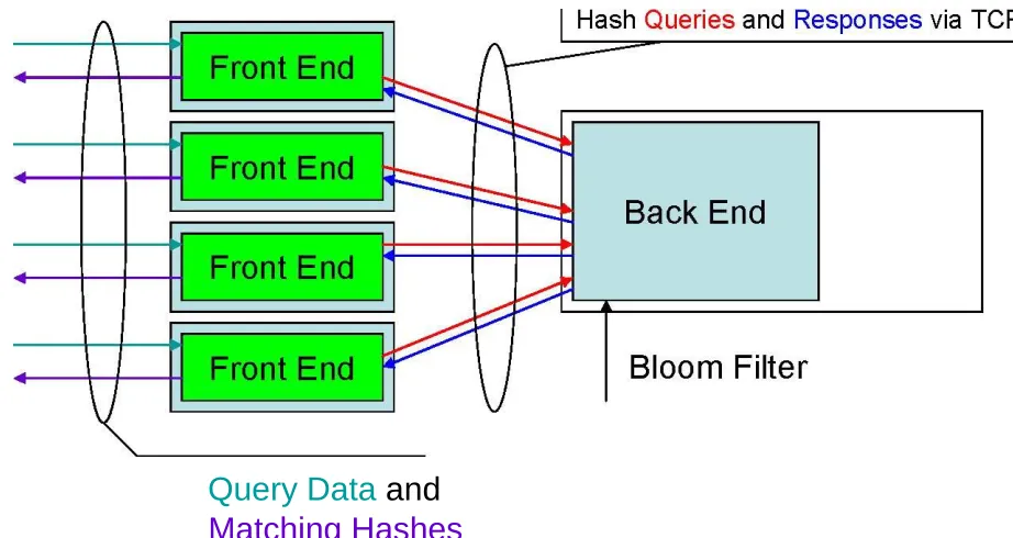
3.2.4 Multiple Servers

Since data correlation is one of the main uses of our tool, we provide a simple way

to query many filters with one set of data to correlate the suspect data set to filters

that have already been created from data used in previous cases. Once all the

back-ends are up and running, which may or may not be on the same physical

server, a specialized front-end can be loaded, that can send the hashes it generates

to many different servers simultaneously. Just as before, many different

of how many hashes matched in each filter. This provides statistical filtering to

the investigator which provides the means to select results with a desired statistical

significance and to determine which filter is most closely related to the hashes of

the data fed to the front-end.

Hash Queries and Responses

Query

Bloom Filters

3.2.5 Filter Comparison

3.3 Implementation Details

Multithreading allows md5bloom the ability to effectively utilize dual core processors, to speed up requests and responses significantly. Since Bloom filter generation from data streams tends to be I/O-bound, the generation options are single threaded. The Bloom server, or daemon, is

multithreaded at two layers. As any TCP/IP server, there is a pool of threads created to handle many connections from many different clients. In addition to the connection queue that TCP/IP stacks provide, the thread pool implementation has a blocking queue to keep track of waiting connections. These connections are established with the client, waiting for one of the available threads to process its requests. The second layer of multithreading is for each client’s requests. Each thread in the

pool of connection threads has its own pool for querying the Bloom filters. Each MD5 hash query that is sent to the client is delegated to this pool separately. The quick, single-client ―server‖ also uses this last level of multithreading, but it obviously does not need the connection thread pool, as it only has one client, itself. That eliminates the costly TCP/IP overhead when it is not necessary to share between multiple clients.

considered an independent hash function. The number of subhashes the MD5 hash is divided

into is determined by the smallest of the values mentioned above. This is because the sizes of the numeric data types in C are 8, 4, 2, and 1 byte. Then, to put the subhashes in the correct range, so that the maximum range of each subhash equals the number of bits in the filter, the subhashes usually need some of the bits masked out. The number of bits to mask is determined by l where m = 2l . For example, if k = 4 and l = 8, there are 32 bits in each subhash, but the size of the filter in bits only fits in 8 bits. To put the subhash in the correct range, the 24 highest bits need to be masked out. Once the subhashes are in the correct range, then a macro is used to set the bit positions in the filter specified by each subhash to 1. If the value of the bit is already 1, then the bit is not changed.

Also, Bloom filter queries only require k bit lookups, where k is the number of hash functions. The bits to be tested are selected in the same manner as the insertion process. A hash table lookup can entail much iteration to even reject the hash, whereas just one of the bits in the bit lookups that are done on the Bloom filter has to be 0. Therefore, the best case to reject a hash for membership in a Bloom filter is one bit lookup, and the worst case is k lookups.

3.4 Command line options

3.4.1 Filter Generation Options

-genstream <l> <k> <r> <block_size> [-daemon port]

This option reads data from standard input in increments specified by the block_size, and

generates MD5 hashes from each of these blocks. These hashes are then inserted into a Bloom filter created using the first three parameters, l, k, and r. These parameters are used in every generation options. The parameter l specifies the size of the filter in bits; the generated filter will contain 2l bits. This also determines how much each subhash is masked out to make sure the range of the subhash values is the same as the range of bit positions in the Bloom filter. The parameter k determines the number of subhash values that are used to set bits in the filter. If the number of subhashes is too high for the size of the filter, md5bloom will display an error, and no Bloom filter will be generated. For example, if k=8and l>16, an error will be returned because at k=8, the hash is broken into 8 16-bit fragments, so l=16 is the maximum filter size for k=8. The parameter ris the ratio m/n that

determines how many hashes can be put into the filter. This means that the maximum number of hashes that can be put into the Bloom filter is floor(m/r). If this number is exceeded, the utility creates a new filter to accommodate the additional items. This should generally be avoided, as search and reject times increase linearly with the number of Bloom filters that must be queried. Therefore, the values of land rshould be chosen carefully to ensure only one Bloom filter is created, and the

-genmd5 <l> <k> <r> [-daemon port]

This option is identical to the previous option, except that the input is expected to be a list of MD5 hashes in a hexadecimal text representation. There should be one hash one each line. All the options have an identical effect, including the –daemonoption, which controls whether the filter is output or if it becomes a server.

Here is an example command line:

md5bloom –genmd5 13 4 8 –daemon 2000

In this case, a Bloom filter is generated with a filter size of 213 or 8192 bits. The 4 indicates that we split the 128-bit MD5 hashes read from standard input into 4 subhashes. Since the filter size is 213, the range of the subhashes must be [0, 213-1]. To put the subhashes, which are 32 bits in this case, in this range, we must mask out the 19 high bits. Once we mask out these bits, the values are then used as an offset into the bit array, and the bits at these offsets are set to 1. The 8 is the bit per element ratio, so the maximum number of elements that can be put in the filter is 8192/8 or 1024. If more than 1024 elements are in the input, then an additional 8192-bit filter is created. This happens at every multiple of 1024 elements. Once all the elements are read, the generated filters are then fed to a daemon, and this daemon begins listening on port 2000. If the daemon option is not specified, all filters generated are output to standard output. For further examples, refer to the chapter on

experiments (Chapter 4).

The following option is used for generating filters from the contents of directories:

-gendir <dir_name> <l> <k> <r> [-daemon port]

Every file in the specified directory is read, an MD5 hash is generated for each file, and then insert into a Bloom filter with the specified parameters. Again, the –daemon only affects the

The next option is used on object files:

-genobj <file_name> <l> <k> <r> [-daemon port]

This option uses the BFD (Binary File Descriptor) library [1] to separate the specified executable, object, or library archive file into sections, generate MD5 hashes from these sections, and insert them into a Bloom filter with the specified parameters. The –daemonoption once again has the same effect.

The following options are used to add data to an existing filter. The specified file is not modified; the new filter with the added data is output to standard output. The –daemonoption can be used with these as well. -addstream <bloom_filter_file> <block_size> [-daemon port] -addmd5 <bloom_filter_file> [-daemon port] -adddir

<bloom_filter_file> <dir_name> [-daemon port] -addobj

<bloom_filter_file> <file_name> [-daemon port] These options work similar to

the aforementioned options. The existing filter is used, so the Bloom filter parameters are not needed; they are read from the file. As before, if the number of items in the filter exceeds m/r, then a new filter will be added to the filter file.

-genclient <l> <k> <r> <port>

This option creates a Bloom filter with the specified parameters, but instead of reading data locally, it is initially empty and listens on the specified port for requests to add hashes to its filter. Like the daemons started with the other options, it also accepts queries for its Bloom filter.

The next option is usually the second step in the process of creating and querying filters.

-load <port> [number_of_threads]

insert or query requests to the Bloom filter. The second parameter is optional and determines the

number of threads for the connection thread pool. This essentially determines how many clients can simultaneously have their requests serviced by the daemon. If it is not specified, the default value is 5. The queue for the connection thread pool is set to twice the number of threads. For example, with the default number of threads, 5 clients can be serviced; while there can be 10 clients in queue waiting to be serviced. Any additional clients must wait in the TCP/IP stack’s connection

queue.

3.4.2 Client options

We provide client options to either add hashes to a Bloom filter server or to query a Bloom filter server with hashes that are very similar to the ―-add‖ and ―-gen‖ options. This allows

much flexibility for comparing various types of data.

-clientstream <host> <port> <block_size>

This option, along with all the other following ―-client‖ options, sends hashes to a Bloom filter server

at the specified hostname and port number. This option creates MD5 hashes from standard input in chunks of data whose size is specified by the block size, and then sends the hashes to the Bloom filter server. -clientmd5 <host> <port> -clientdir <host> <port> <dir_name>

-clientobj <host> <port> <obj_name> These options read data and generate hashes in an

identical way to their ―-gen‖ and ―-add‖ counterparts, but instead of adding the hashes to a local

Bloom filter, they send the hashes to the Bloom filter server specified by their hostname and port number.

These options below perform the most important function in this utility, querying the

Bloom filters. The first set of options communicates with a remote Bloom filter server via TCP/IP; whereas the second set queries a local Bloom filter without the need for a separate server.

-querystream <host> <port> <block_size>

-querymd5 <host> <port> -querydir <host>

<port> <dir_name> -queryobj <host> <port>

<obj_name>

These options generate hashes in the same manner as their ―-gen,‖ ―-add,‖ and ―-client‖ counterparts, but these functions query a remote Bloom filter server. Hashes that are contained in the remote Bloom filter are displayed in hexadecimal string format to standard output. The ―querymd5‖

function is useful as a filter for MD5 hashes, as it reads and writes in the same format and outputs only matching hashes. These options are used when there is a need for multiple clients to be able to query a Bloom filter concurrently.

-queryfilterstream bloom_filter_file block_size

-queryfiltermd5 bloom_filter_file -queryfilterdir

bloom_filter_file dir_name -queryfilterobj

bloom_filter_file obj_name

3.4.4 Comparison options

-diff filter_file_1 filter_file_2

This option performs bitwise comparisons of the Bloom filters. For the comparison to work, the m, or number of bits, of the filters must be equal. Also, the number of hash functions, k, must be equal as well. If they are not, then the results that this option returns are not meaningful. The output for this option is the number of matching bits, that is, the number of bits set to 1 in both filters in the same position, the number of bits set to 1 in the first filter, and the number of bits set to 1 in the second filter. Please refer to section 4.1.2 for some example runs of this option.

-comp filter_file_1 filter_file_2 [–p <p_min> <p_max>]

Chapter 4: Experimental Evaluation

To prove the accuracy and usefulness of this tool, we performed some experiments to verify the analytical work we mentioned in section 2.1.1. We also show some benchmarks that we ran against our tool to display its efficiency compared to other commonly used tools. Also, we showed some sample uses to demonstrate its usefulness.

We verify the mathematical formulae we presented in chapter 2 for false positive rates for various (Bloom) filter parameters and the matching bit probability, which is a key element in proving or disproving similarity of the data used to create the filters. The results of these verifications are important as both of these formulas are needed to interpret the values returned by md5bloom.

Verifying the false positive rates for the filters is important, because if the false positives rates are too high, any performance gains would be meaningless as the results would be useless. Without a valid formula to determine whether a certain number of bits happen to match by chance in a filter, there would be no way to determine if the data used to create the filters were similar.

We conduct various experiments to demonstrate the performance gains we achieve compared to other utilities. To demonstrate its usefulness, we show the tool’s ability to identify similar items quickly, by using the statistical information provided by the ―-comp‖ option. We also show that

filter comparison can more than just show similarity, but the level of similarity.

4.1 Verification

number of hashes printed by the client when the filter used is generated from random data and

another set of random data is used to query the filter. If the files are truly random, any matches should be false positives. To test the matching bit probability density function (PDF), we generate two random sets of data, generate filters from them, and use the ―-diff‖ option to md5bloom to get the

number of matching bits. The values returned should fall under the curve of the PDF for the specified filter parameters.

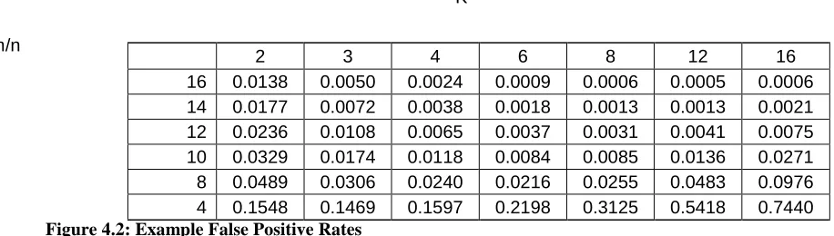
4.1.1 False Positive Rate Verification

Recall from Chapter 2, the expression for the false positive rate for a Bloom filter: ⎛⎞k P_fp =⎜1 − ⎛⎜1 −

1 ⎟⎞

kn

⎟_{≈ (1 −} e−kn / m )k _⎜⎟

⎝ m ⎠

⎝⎠ _{Equation 4.1: False Positive Rate}

Therefore, for n = 128, m = 1024, and k = 4, Pfp = 0.0240. In this case the ratio r used is 8

(1024/128). To verify this false positive rate, I generated 10 random files of size 65,536 bytes (128 * 512 byte blocks) and generated 10 filters, one for each file, by running the following command:

md5bloom –genstream 10 4 8 512 < random_data_file > filter_file

Once the filter files were created, we queried all 90 pairs of filter and data files by running the following command:

md5bloom –queryfilterstream filter_file 512 < random_data_file

The average number of matching hashes that was measured across the 90 trials was 2.8556. For n = 128, this gives an experimental false positive rate of 0.0223, which is slightly less than the

same amount of items used to create the filter is used to query the filter. If not, the false positive rate is relative to the amount of hash queries that are posed to the Bloom filter.

K

m/n

Figure 4.2: Example False Positive Rates

4.1.2 Matching Bit Probability Verification

To verify the normal distribution approximation mentioned in section 2.1.1, we generated 1,000 random data files, 65 kilobytes in size. We then generated 1,000 filters from each of these random files, using a block size of 512 bytes and 4 hash functions. This setup results in the following parameters: m=1024, n1=128,n2=128, and k=4. From these parameters, and the normal distribution approximation stated above, the mean of this distribution should be 158.53, and the standard deviation should be 11.58. This corresponds to the middle curve in Figure 1. The 1,000 filters give us 499,500 unique comparisons. With this data set, the calculated mean is 158.94, and the calculated standard deviation is 8.73.

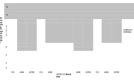
4.2 Performance Results

For comparison of md5bloom’s performance, we compared the open-source package md5deep. This tool has many similar options to our tool but quite a different implementation. md5deep does not return false positives as our tool does, but since the false positive rates are quantifiable, the performance gains we achieve, especially on large hash sets, are very likely to make up for any false positives our tool may return.

2 3 4 6 8 12 16

In addition to the shorter processing times, the file sizes for the files that store our Bloom

filters are substantially smaller than the lists of hashes used by md5deep to perform its matching. Since both md5bloom and md5deep are I/O-bound particularly in the generation step, this contributes significantly to the slowness of md5deep. Since the MD5 implementations are substantially the same, the only reason md5deep is slower is the amount of data written to standard output for the generation of the hash sets. Since the amount of data that has to be read in the comparison step by md5bloom is significantly less than md5deep, the larger file sizes also slow down the hash matching step.

Not only do the file sizes affect the performance of these tools, the memory footprint of the data structures used to store the hashes in memory by md5deep have a significant potential to slow down the hash queries. It uses a hash table to store all the hashes in memory, whereas the Bloom filters used by md5bloom can reduce the amount of memory required to store an equivalent size hash set. How much reduction can be achieved is dependent on the ratio chosen for the filter. This reduction can allow less powerful workstations do hash comparisons in much less time, due to the lower memory footprint, which lessens the possibility of virtual memory usage, which can slow the

processing time to a crawl. More importantly, however, this can allow more powerful workstations compare much larger hash sets, without taking hours or days of processing time.

Generating hash sets is usually the first step in comparing data sets, unless hash sets are provided. To use the tool we developed, md5bloom, or md5deep, a hash set must be generated to be able to

md5bloom is less than the time md5deep takes to generate identical size hash sets, mainly for

larger hash sets.

To demonstrate this performance advantage, we compared the time both md5bloom and md5deep required to generate hash sets with different block sizes. We also tried to eliminate the effects of the I/O that is inherent in both tools. We eliminated the input I/O by ensuring the input files were cached. We accomplished a similar effect on output by directing the output to ―/dev/null.‖ With both of these

methods in place, we effectively isolated the I/O time from the CPU time, as much as practical. We tested all possible combinations of this to pinpoint the main bottleneck in the md5deep tool. We expected to see very similar processing time values between the two tools when I/O is eliminated completely, md5deep to be slightly higher than md5bloom with caching and eliminating writing data to the hard drive, and md5deep to be significantly slower when all I/O is done.

To perform these tests, we generated a random data file, 128 megabytes in size. With block sizes of 512, 4096, and 32768 bytes, this created hash sets of sizes 262144, 32768, and 4096,

respectively. These hash sizes were chosen for the following reasons: 512, current hard drive sector sizes, 4096, the future standard sector size for hard drives, and 32768, generally the largest cluster size used under NTFS.

To ensure caching was done on these tests, we ran one test with the following command:

time md5bloom –genstream 21 4 8 512 < rnd1 > /dev/null

This copied the file to the workstation’s memory disk cache, which eliminates the need for disk I/O

time md5deep –p 512 rnd1 > /dev/null

A similar method is used to ensure caching in running this command. Notice at the end of both commands is output to /dev/null. This prevents output to disk, which eliminates the rest of the

I/O in this method.

For the tests done without caching, 10 different random 128 megabyte files were created. Each trial of the test iterated over the 10 files, effectively forcing a purge of the disk cache due to the machine having only 512 MB of RAM. To do the hard drive output, /dev/null is simply replaced with a

valid regular file name, either existing or non existing.

No Output / No Output / File Output / File Output / Input Cached Input Not Cached Input Not Cached Input Not Cached

Pr oc es sin g Ti me (S ec on ds )

We performed all these tests and discovered some interesting results. (Figure 4.3) When hash sizes were only 4096, md5deep performed slightly better on average, except when the

18 16 14 8 1 0 1 2 md5bloom md5deep 6 4 2 0

512 4096 32768 512 4096

32768 512 Block Size

4096 32768 512 4096 32768

results were output but the data file was cached. Also, with hash sets of size 32768, when output

is directed to /dev/null, md5deep is slightly better than md5bloom. But for 262,144 size hash

sets, md5bloom was significantly faster than md5deep in all 4 test combinations. For the remaining tests, md5bloom was slightly faster that md5deep.

The results of these tests indicate two things. One, md5bloom performs better on large hash sets. We expect the performance gap to widen with even larger hash sets. Two, when I/O is eliminated, except for large hash sets, md5deep performs better than md5bloom. However, eliminating I/O is not possible if matching is to be done with the results. There is no real point to using either of these tools without matching against other hash sets. So, overall, md5bloom is the better performer when it comes to generating hash sets.

4.3 Similarity Experiments

The ―-comp‖ option described in Chapter 3 is the option we used to perform these experiments. We chose the ―-comp‖ option because we needed statistical analysis of the number of matching bits

To demonstrate the utility of Bloom filters to detect similarity between data sets, we

decided to compare files from different versions of a Linux distribution. The distribution we chose was the KNOPPIX distribution, because it is a bootable Linux distribution, bootable directly from CD. Installation on a hard disk is not necessary, which facilitates the ability to work with the distribution quickly. Since the file system on the CDROM is read only, subsequent accesses are guaranteed to have the same results. Other distributions give choices as to which packages to install, whereas KNOPPIX is a consistent distribution, where all utilities are automatically included, to reduce the level of variation due to utilities not being included in different versions.

4.3.1 Similarity of /usr/bin in KNOPPIX versions

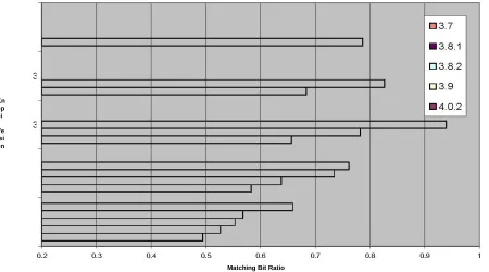
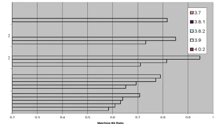
The first test we did to demonstrate the usefulness of md5bloom in detecting similarity is to compare the hashes of all the binary files in six different versions of KNOPPIX. The versions we chose were 3.6, 3.7, 3.8.1, 3.8.2, and 4.0.2. To perform this test, we ran the following commands after booting each version of KNOPPIX: md5bloom –gendir /usr/bin 15 4 8 >

knoppix<version>-8.bf md5bloom –gendir /usr/bin 14 4 4 >

knoppix<version>-4.bf md5bloom –gendir /usr/bin 13 4 2 >

knoppix<version>-2.bf We originally ran the first two sets of commands, and all the filter

bits per element that we were able to tell that the versions were definitely similar, we decided to

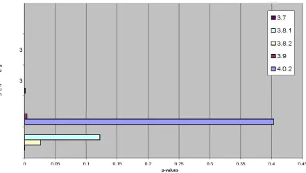
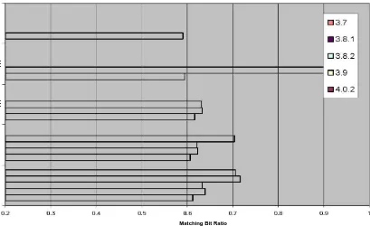
try an even smaller bit per element ratio of 2. We still found a linear relationship between the versions (Figure 4.6), but we are less confident about their similarity. In the two previous tests, the p-values, or confidence levels, were nearly 0, which means that it is nearly impossible for the number of bits that matched to match by chance, however, for r=2, the p-values (Figure 4.7) were higher. The number of elements on all these versions was approximately 2,000. So for n≈2000, r=4, the lowest level of compression that can be used to determine similarity definitively.

Knoppix /usr/bin m = 32768 m/n = 8 k = 4

Kn op pi x Ve rsi on

3.9

3.8.2

3.8.1

3.7

3.6

Matching Bit Ratio

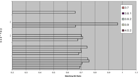
Knoppix /usr/bin m = 16384 m/n = 4 k = 4

3.9

3.8.2

3.8.1

3.7

3.6

Matching Bit Ratio

Figure 4.5: KNOPPIX /usr/bin comparison / r = 4 Kn

op pi x Ve rsi on Kn op pi x Ve rsi on

3.9

3.8.2

3.8.1

3.7

3.6

Knoppix /usr/bin m = 8192 m/n = 2 k = 4

Kn op pi x Ve rsi on

3.9

3.8.2

3.8.1

3.7

3.6

p-values

Figure 4.7: KNOPPIX /usr/bin comparison p-values / r = 2

4.3.2 Similarity of the standard C library (libc) in KNOPPIX versions

The next test we did to demonstrate md5bloom’s capability to detect similarity is to compare the similarity of the standard C library (libc) in six different KNOPPIX versions, the same ones we chose for the previous test. In this test, we used the option that hashes object files by section by running the following commands: md5bloom –genobj /lib/libc.so.6 9 4 8 >

knoppix-<version>libc-1.bf md5bloom –genobj /lib/libc.so.6 8 4 4 >

knoppix-<version>libc-2.bf md5bloom –genobj /lib/libc.so.6 10 4 16 >

knoppix-<version>libc-3.bf We initially ran the first two sets of commands under each

(Figure 4.9) tests the libc’s in version 3.8.2 and 4.0.2 were nearly exactly the same. Once we

discovered this, we checked the release dates of 3.8.2 and 4.0.2, and we found that they were released 22 days apart, where all the other versions were at least 3 months apart. This would be expected as there would not be many patches to the stable version of libc within 22 days.

One thing different we detected in this test is that unlike the previous testing the linear relationship of the matching bit ratios to the versions was not present (Figure 4.8). We suspected that since there was such a small number of elements (~50), even the compression done at r=8 was too high to show a definitive linear relationship, so we decided to try r=16 (Figure 4.10). Interestingly enough, the relationship across the versions was not exactly linear, but it was closer than the other compression levels. Given these results, it is safe to assume that relationships will continue to trend more linear as r increases, or the compression rate decreases.

Knoppix libc m = 512 m/n = 8 k = 4

Kn op pi x Ve rsi on

3.9

3.8.2

3.8.1

3.7

3.6

Matching Bit Ratio

Knoppix libc m = 256 m/n = 4 k = 4

3.9

3.8.2

3.8.1

3.7

3.6

Matching Bit Ratio

Figure 4.9: KNOPPIX libc comparison / r = 4 Kn

op pi x Ve rsi on Kn op pi x Ve rsi on

3.9

3.8.2

3.8.1

3.7

3.6

Knoppix libc m = 1024 m/n = 16 k = 4

Matching Bit Ratio

Chapter 5: Conclusions

5.1 Summary

Bloom filters can be an effective tool in filesystem forensics. It can alleviate scalability problems by compressing hash digests into a much smaller space. For acceptable performance and reliability, experiments have shown that compression in the range of 8-32 times yields excellent performance and reliablity. Bloom filters are also effective as data structures to organize hashes, which serves to facilitate statistical analysis of content comparisons to provide a better mechanism than whole file hashing to identify similar data instead of identifying only identical data.

We developed a framework to use filters as a whole for comparison and analysis, instead of using individual hash queries that all known previous published papers have used. We provided a means to compare filters directly and provided statistical means to analyze the data from these comparisons. From the data analysis, we can reliably identify similar sets of data, and provide a measure of

confidence in the similarity of these data sets.

provide an efficient means of identifying similarity without a user having to do calculations.

This tool can be effective as a standalone tool to identify data similarity, or as a component of an investigators toolbox to provide hints or leads to allow them to discover data that might have taken much more time to identify with existing tools.

We demonstrated the efficiency of our tool by running performance comparisons against a common used tool with similar functionality, md5deep [6]. We noticed significant performance gains by using our tool over md5deep, particularly on large hash sets. Our tool was approximately equal in

performance with md5deep with smaller hash sets, so in practice we achieve greater performance gains with large hash sets. Our statistical analysis of direct comparisons was put to work in identifying similar data in six different versions of KNOPPIX. It provided an expected linear relationship in the similarity of binary files between versions and the nearly similar binary files between minor versions of KNOPPIX, particularly 3.8.1 and 3.8.2. We showed the utility of doing fine-grained hashing on object files by comparing the standard C libraries between versions of KNOPPIX. We did not discover a linear relationship at higher levels of compression, but at lower levels of compression the linear relationship became clearer. We were able to identify two versions of KNOPPIX as being released a short time apart (22 days) by finding a nearly identical standard C library between versions 3.8.2 and 3.9.

5.2 Future Work

The front-end mentioned in section 3.2.4 has not yet been implemented, but we plan to implement it in the future. We expect the option to be invoked as follows: -filtersearchstream

list_of_filters block_size < data -filtersearchmd5 list_of_filters <

-filtersearchobj list_of_filters obj_name

The list of filters should be a list of either filenames or hostname:port combinations. There is no reason, unless some implementation details prevent it, to limit the list to only local files or to only remote filters. This would allow comparisons to shared filter servers and local servers

simultaneously.

References

[1] LIB BFD, the Binary File Descriptor Library.

<http://www.gnu.org/software/binutils/manual/bfd-2.9.1/html_mono/bfd.html>. [2] Bloom, Burton H. ―Space/time tradeoffs in hash coding with allowable errors.‖ Communications of the ACM (1970); 13(7):422-6.

[3] Broder, Andrei and Michael Mitzenmacher. ―Network applications of bloom filters: a survey.‖ Internet Mathematics (2005); 1(4):485-509.

[4] Garfinkel, Simson L. ―Forensic feature extraction and cross drive analysis.‖ In: Proceedings of the Digital Forensic Research Workshop (2006).

[5] Kornblum, Jesse. ―Identifying almost identical files using context triggered piecewise hashing.‖ In: Proceedings of the Digital Forensic Research Workshop (2006).

[6] Kornblum, Jesse. md5deep. <http://md5deep.sourceforge.net>.

[7] Manber, Udi. ―Finding similar files in a large file system.‖ In: Proceedings of the USENIX Winter 1994 Technical Conference; January 1994, 1–10.

[8] Mitzenmacher, Michael. ―Compressed bloom filters.‖ IEEE/ACM Transactions on Networks, October 2002; 10(5):613–20.

[9] National Software Reference Library. National Institute of Standards and Technology. <http://www.nsrl.nist.gov>.

[10] Patterson, David A. ―Latency lags bandwidth: Recognizing the chronic imbalance between bandwidth and latency, and how to cope with it.‖ Communications of the ACM (2004); 47(10): 71-75.

Vita