University of New Orleans University of New Orleans
ScholarWorks@UNO
ScholarWorks@UNO
University of New Orleans Theses and
Dissertations Dissertations and Theses
Summer 8-5-2019
General Nonlinear-Material Elasticity in Classical One-Dimensional
General Nonlinear-Material Elasticity in Classical One-Dimensional
Solid Mechanics
Solid Mechanics
Ronald Joseph Giardina Jr
University of New Orleans, [email protected]
Follow this and additional works at: https://scholarworks.uno.edu/td
Part of the Analysis Commons, Applied Mechanics Commons, Civil Engineering Commons, Engineering Mechanics Commons, Mechanics of Materials Commons, Other Applied Mathematics Commons, Other Mathematics Commons, Special Functions Commons, and the Structural Materials Commons
Recommended Citation Recommended Citation
Giardina, Ronald Joseph Jr, "General Nonlinear-Material Elasticity in Classical One-Dimensional Solid Mechanics" (2019). University of New Orleans Theses and Dissertations. 2666.
https://scholarworks.uno.edu/td/2666
This Dissertation is protected by copyright and/or related rights. It has been brought to you by ScholarWorks@UNO with permission from the rights-holder(s). You are free to use this Dissertation in any way that is permitted by the copyright and related rights legislation that applies to your use. For other uses you need to obtain permission from the rights-holder(s) directly, unless additional rights are indicated by a Creative Commons license in the record and/ or on the work itself.
General Nonlinear-Material Elasticity in Classical One-Dimensional Solid Mechanics
A Dissertation
Submitted to the Graduate Faculty of the University of New Orleans
in partial fulfillment of the requirements for the degree of
Doctor of Philosophy in
Engineering and Applied Sciences Mathematics
by
Ronald Joseph Giardina, Jr.
B.S. University of New Orleans, 2010 M.S. University of New Orleans, 2013 Certificate University of New Orleans, 2016
M.S. University of New Orleans, 2017
With all my love
this dissertation is dedicated to my parents,
Acknowledgements
This document and the degree it represents is a result of the efforts of many people, all of
whom I could not hope to individually recognize upon this page, so I would like to thank all
of my friends and family who have helped me pursue this goal. I would specifically like to
thank a few friends and colleagues – Jonathan Joseph, Rosa Fustera, Jonathan Redman, and
Lance Lacoste – who helped me organize my ideas and my thoughts into a more presentable
and understandable manner. I would also like to thank the University of New Orleans for
funding my scholarship, and specifically Amanda Athey and the rest of the Graduate School
whose help and support over the years have led to this moment.
I owe thanks to Dr. Kenneth Holloday for the breadth of his advice and frequent
con-versations. I am similarly indebted to Dr. Juliette Ioup for her suggestions and continual
encouragement, and Dr. Alex McCorquodale and Dr. Norma-Jean Mattei for their guidance
and practical mechanical insights. I likewise owe a great deal of thanks to Dr. Ralph
Sax-ton who offered counsel and continually challenged my understanding making me a better
researcher. I also owe thanks to Dr. Jairo Santanilla, who offered me his help when I needed
it, as well as everyone else in the Department of Mathematics and the Department of Civil
Engineering who have contributed to my academic growth.
Finally, I wish to express my most sincere gratitude to my advisor and mentor Dr.
Dongming Wei, without whom I would never have embarked on this long and fulfilling
Contents
List of Figures . . . vii
List of Tables . . . xii
Nomenclature. . . xiii
Abstract . . . xiv
1 Introduction . . . 1
1.1 Generalized Sine and Cosine . . . 1
1.2 Ramberg and Osgood . . . 8
2 Generalized Ellipses . . . 19
2.1 Continuity . . . 22
2.2 Distance . . . 26
2.3 Ordinary Differential Equations . . . 31
2.3.1 Existence and Uniqueness . . . 35
2.4 Properties of the Generalized Ellipse . . . 40
2.4.1 Defining the Period . . . 45
2.5 Examples of Continuous, Periodic Functions . . . 51
3 The General Bending Moment . . . 59
4.1 The Euler Model . . . 70
4.2 Axially Loaded Euler-Column Buckling . . . 73
5 Numerical Examples and Validation . . . 78
5.1 Perpendicularly Loaded Beam-Column Members . . . 78
5.2 Axially Loaded Beam-Column Members . . . 83
Bibliography . . . 87
Appendix . . . 98
A Mechanics . . . 98
A.1 Curvature . . . 98
A.2 Euler Columns . . . 102
B Properties of Functions . . . 104
B.1 Convexity and Concavity . . . 104
B.2 Antiperiodicity . . . 105
B.3 Inverse Functions . . . 105
B.3.1 Differentiation . . . 105
B.3.2 Homogeneity . . . 106
B.4 Monotonic Functions . . . 107
B.4.1 Unimodal Functions . . . 107
B.4.2 Differentiability . . . 107
B.5 Existence Theorems . . . 107
B.6 Uniqueness Theorems . . . 109
B.7 Continuation of Solutions . . . 110
B.8 n-ellipse . . . 111
C.1 Banach Spaces . . . 112
C.1.1 Birnbaum-Orlicz Spaces . . . 112
List of Figures
2.1 A graphical representation of the bounded behavior of the curve over the plane
about a point in each quadrant. For someδ-ball defined over UF andUGthere
must be somex, y pairs within the shaded regions. . . 24
2.2 A graphical representation of the bounded behavior of the expansion and
contraction of the curve over the plane about a point in each quadrant. . . . 26
2.3 Figure 2.3a plots a high growth F(x) and Figure 2.3b plots the inverse of H.
Each of these plots show the effect of the growth of the curve on the values
used in the distance function (2.16). . . 29
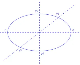
2.4 The discernible values of y along the circumference of the generalized ellipse
based on the known symmetries generated by F and G. . . 47
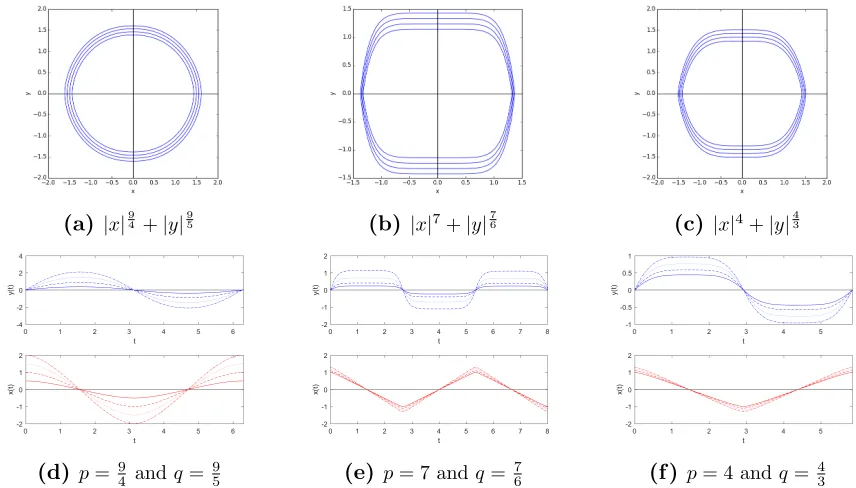
2.5 Plots of y(t) and x(t) and their associated generalized ellipses for power-law
systems which satisfy Conjecture 1. Figures 2.5d and 2.5a are plotted for
initial conditionsx0 = 0.5,1,2,3, Figures 2.5e and 2.5b, and Figures 2.5f and
2.5c are plotted for initial conditionsx0 = 1,1.1,1.2,1.3. . . 49
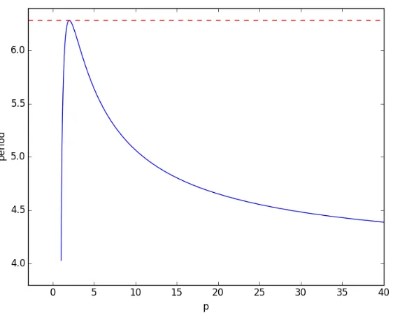
2.6 A plot of the invariant periods forLp spaces which satisfy Conjecture 1. . . . 50
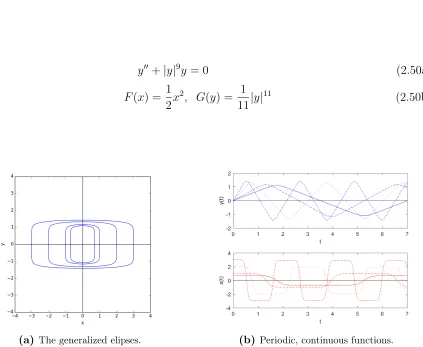
2.7 Plots of the system defined by (2.50) with parametersb = 0, a= 0.7071, 1, 2,
and 3, which correspond to the generalized ellipses starting from the middle
going out. The plots at the top on the right are the curvesy(t) and the plots
on the bottom are x(t) with the initial conditions corresponding to the solid
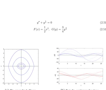
2.8 Plots of the system defined by (2.51) with parametersb = 0, a= 0.7071, 1, 2,
and 3, which correspond to the generalized ellipses starting from the middle
going out. The plots at the top on the right are the curvesy(t) and the plots
on the bottom are x(t) with the initial conditions corresponding to the solid
line, dashed line, dotted line, and dash-dot line, respectively. . . 52
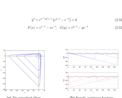
2.9 Plots of the system defined by (2.52) with parameters b = 0, a = 2.0074,
3.42113, 3.79709, and 4.0789, which correspond to the generalized ellipses
starting from the middle going out. The plots at the top on the right are the
curves y(t) and the plots on the bottom are x(t) with the initial conditions
corresponding to the solid line, dashed line, dotted line, and dash-dot line,
respectively. . . 53
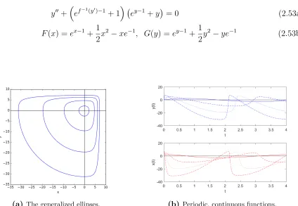
2.10 Plots of the system defined by (2.53) with parameters b = 0, a = 2.21336,
4.70527, 6.20952, and 7.16741, which correspond to the generalized ellipses
starting from the middle going out. The plots at the top on the right are the
curves y(t) and the plots on the bottom are x(t) with the initial conditions
corresponding to the solid line, dashed line, dotted line, and dash-dot line,
respectively. . . 54
2.11 Plots of the system defined by (2.53) with parameters b = 0, a = cosh 3 ≈
10.06766, cosh 5≈ 74.2099, cosh 8 ≈1490.47916, and cosh 12≈ 81377.39571, which correspond to the generalized ellipses starting from the middle going
out. The plots at the top on the right are the curvesy(t) and the plots on the
bottom arex(t) with initial conditionsx0 = 3,3.5,4,4.5 corresponding to the
2.12 Plots of the system defined by (2.55) with parameters b = 0, a = √6, √10, 3√2, and 2√6, which correspond to the generalized ellipses starting from the middle going out. The plots at the top on the right are the curves y(t) and
the plots on the bottom are x(t) with the initial conditions corresponding to
the solid line, dashed line, dotted line, and dash-dot line, respectively. . . 56
2.13 Plots of the system defined by (2.56) with parameters b= 0, a= 0.5, 0.7, 0.9,
and 1.1, which correspond to the generalized ellipses starting from the middle
going out. The plots at the top on the right are the curvesy(t) and the plots
on the bottom are x(t) with the initial conditions corresponding to the solid
line, dashed line, dotted line, and dash-dot line, respectively. . . 57
3.1 A beam-column element with length L, neutral axis coincident with the x
axis, and cross-section with heightH along the y axis and widthB along the
z axis. . . 60
3.2 We plot the linear stress-strain relationship, the associated special function
ψ, and the internal bending moment for a Young’s modulus of E = 193,054
Pascals, and rectangular cross-section with B = 0.00635 meters and H =
0.00635 meters. . . 64
3.3 We plot the nonlinear stress-strain relationship, the associated special function
ψ, and the internal bending moment for a nonlinear power-law Hollomon
material with material coefficient K = 4.92, strain-hardening exponent m =
0.15823, and rectangular cross-section with B = 0.00635 meters and H =
0.00635 meters. . . 65
3.4 We plot the nonlinear stress-strain relationship, the associated special function
ψ, and the internal bending moment for a nonlinear Ramberg-Osgood material
4.1 A staticly deflected simply supported beam with a rectangular cross section
of heigh H, width B, length L, and neutral axis parametrized bys. . . 67
4.2 Figure 4.2a is a combined loading with an evenly distributed load w across
the length of the beam and a point load P perpendicular to the beam at its
center. Figure 4.2b is an axial point loadP applied at the right support. The
left support represented by a triangle is fixed both vertically and horizontally,
but is allowed to rotate freely. The right support represented by a circle is
fixed vertically but is allowed to move horizontally and to rotate freely. . . . 68
4.3 A staticly deflected cantilever beam with a rectangular cross section of heigh
H, widthB, length L, and neutral axis parametrized bys. . . 69
4.4 A combined loading of a cantilever beam with an evenly distributed load w
across the length of the beam and a point load P applied at the free end of
the beam at an anlge α. The left support represented by slanted lines along
a wall is fixed vertically, horizontally, and rotationally. The right end of the
beam is allowed to move freely. . . 69
4.5 The force P projects the equilibrium state (solid line) through the potential
deflected positions of the member (dashed lines) from the at rest position to
the specific deflected position. . . 77
5.1 A comparison of the displaced cross section of the beam using linear Youngs
material model and the Ramberg-Osgood material model for varying end
loads. Plots were constructed using Python. . . 81
5.2 A comparison of the displaced cross section of the beam using linear Youngs
material model, nonlinear Hollomon power law model, and the
Ramberg-Osgood material model. Plots were constructed using Python. . . 82
5.3 A comparison of the displaced cross section of the beam using nonlinear
Hol-lomon power law material model and the Ramberg-Osgood material model
A.1 A diagram of the segmentaiton of a linear section of curvature. . . 98
A.2 A log-log axis plot of the deviation from one in the denominator associated
with values of the slope of w. . . 100
A.3 The change in angle between the tangents, T1 and T2, along an osculating
List of Tables
5.1 A comparison of the magnitude of the measured experimental vertical tip
deflection,δye, with the calculated deflection, δyc, and the currently proposed
method,δy, for a common linear material behavior. . . 79
5.2 A comparison of the calculated vertical and horizontal tip deflections in the
literature,δyc andδxc, with the calculated deflections of the currently proposed
method,δy and δx, for a nonlinear power-law material behavior. . . 79
A.1 We compare the associated values of the change in deflection dwdx and error ε
σ uniaxial stress
σ−1 the inverse of the uniaxial stress function
uniaxial strain
E Young’s modulus
K material modulus for a nonlinear power-law relationship
T the period
fSg the general sine function
fCg the general cosine function
psq the standard form of the general sine function for power-lawf and g
pcq the standard form of the general cosine function for power-law f and g
M the general bending moment
ψ a unique function for each σ which helps define the general bending moment
M−1 the inverse of the general bending moment
M the antiderivative of the inverse of the general bending moment
M−1 the inverse of the antiderivative of the inverse of the general bending moment
κ curvature
I the second moment of area which helps define the linear internal bending moment
Im a general second moment of area used to define a power-law internal bending moment
H cross-sectional height of a rectangular beam
B cross-sectional width of a rectangular beam
L length of a rectangular beam
P point load applied to a beam-column member
Pn, Pcrit critical buckling loads
w distributed load across the length of a member
Abstract
We will create a class of generalized ellipses and explore their ability to define a distance on
a space and generate continuous, periodic functions. Connections between these continuous,
periodic functions and the generalizations of trigonometric functions known in the literature
shall be established along with connections between these generalized ellipses and some
spectrahedral projections onto the plane, more specifically the well-known multifocal ellipses.
The superellipse, or Lam´e curve, will be a special case of the generalized ellipse. Applications
of these generalized ellipses shall be explored with regards to some one-dimensional systems
of classical mechanics. We will adopt the Ramberg-Osgood relation for stress and strain
ubiquitous in engineering mechanics and define a general internal bending moment for which
this expression, and several others, are special cases. We will then apply this general bending
moment to some one-dimensional Euler beam-columns along with the continuous, periodic
functions we developed with regard to the generalized ellipse. This will allow us to construct
new solutions for critical buckling loads of Euler columns and deflections of beam-columns
under very general engineering material requirements without some of the usual assumptions
associated with the Ramberg-Osgood relation.
Keywords— Ramberg-Osgood, Euler beam-column, generalized ellipses, critical buckling
1
Introduction
1.1
Generalized Sine and Cosine
In the last half-century generalized trigonometric functions have experienced an increase
in interest, largely with regard to the study of eigenvalues of p-Laplace expressions. In
recent years there has been demonstrated several applications of these expressions beyond
their strict mathematical study and into the application of these functions to the field of
mechanics. The beginnings of the generalized trigonometric functions can be traced back to
the elliptic integral first studied by Giulio Fagnano, Leonhard Euler, and later by
Adrien-Marie Legendre. A beautifully written history of the development of the elliptic integrals
can be found in [1]. Elliptic functions were first introduced by Niels Henrik Abel who studied
them as the inverses of elliptic integrals. His work would be improved and expanded upon by
Karl Weierstrauss and Carl Gustav Jacobi. These functions are not descriptions of ellipses
as classicaly understood, but elliptic curves. They are called such because much of the early
investigations were in connection to defining the arclength of ellipses. They have found
ubiquitous use in the modern age in cryptography, mechanics, and even played a role in
Andrew Wiles proof of Fermat’s Last Theorem. Many interesting elliptic functions and their
properties have been built out of this work over the interceding two centuries since they were
first described.
The generalized trigonometric functions upon which we shall be expanding share some
relations to the elliptic integrals of the 19th century. While Weierstrauss, Abel, Jacobi, and
others may have played upon the edges of these functions, there is no indication in the
to have gone unrecognized until they were addressed by Erik Lundberg [3] in his 1879 thesis
Unders¨okningar om hypergoniometriska funktioner af komplexa variabla samt om
temper-aturangifvelser, but this work did not see wide dissemination. Lundberg’s contributions to
this field were not even largely known until recently when they were introduced by Jaak
Peetre [4] who found his thesis in a collection of reprints once belonging to Mittag-Leffler.
The only other person known to engage in this subject before the close of the 19th century
was a German secondary school director Ernst Meissel, though his work was almost entirely
unpublished and appeared only in brief notes [5]. Meissel was considered among the greatest
master calculators of his day. Raymond Clare Archibald [6] compared him with Weierstrauss,
Hermann Grassman, and Johannes Tropfke. Jaak Peetre again provides us with an overview
of Meissel’s contributions as well as a scientific biography of his life [5].
After Meissel, work on these functions would again dissappear almost entirely from the
record until it was picked up by David Schelupsky [7] more than 70 years later. In 1959,
Schelupsky published A Generalization of the Trigonometric Functions in which he anchors
a generalization of the traditional sine and cosine trigonometric functions to the second order
ordinary differential systems they solve, which had been studied only briefly in the latter half
of the 19th century. In 1963 Frank David Burgoyne [8] in his very brief paper Generalized
Trigonometric Functions carries on the work of Schelupsky and connects it with the earlier
work of Alfred Cardew Dixon [9], Oscar Sherman Adams [10], and Mariette Laurent [11].
He investigates some differential parametrizations of an expression of the ellipse
x a n + y b n
= 1 (1.1)
which is frequently referred to in the literature as the superellipse, or the Lam´e curve after
Gabriel Lam´e. The superellipse is closely related to the generalized trigonometric functions
as currently studied in the literature.
identifying the existence of eigenvalues and eigenfunctions. This would take a prominent
position in the research into generalized trigonometric functions in the last half of the 20th
century. In 1977 Pavel Dr´abek [12] first considered the existence of eigenvalues and
eigen-functions in relation to these systems in his articleRanges of a-homogeneous Operators and
Their Perturbations. In 1984 Mitsuharu ˆOtani [13] determined explicitly the eigenvalues,
eigenfunctions, and zeros of some nonlinear elliptic equations involving the p-Laplace
oper-ator in his paper A Remark on Certain Nonlinear Elliptic Equations. After ˆOtani, a central
focus of future research into these functions would be the properties of the p-Laplacian.
In 1992 Jaak Peetre [14] would uncover relations between these periodic functions and K
-functionals in his articleThe Differential Equationy0p−yp =±1(p >0). Peter Lindqvist [15]
would closely follow this work with his 1993 paperNote on a Nonlinear Eigenvalue Problem
in which he investigated the relations between eigenvalues of p-Laplace type systems whose
exponents were complex conjugates of one another. Lindqvist would follow this with a more
comprehensive introduction [2] to the theory of generalizing trigonometric functions in his
1995 paperSome Remarkable Sine and Cosine Functions. In their 1999 paperOn the Closed
Solution to Some Nonhomogeneous Eigenvalue Problems with p-Laplacian. Pavel Dr´abek
and Ra´ul Man´asevich [16] would close out the century by characterizong solutions to these
differential systems as inverses of the incomplete Beta function.
Entering into the new millennium Lindqvist and Peetre [17] jointly published a solution
given by Jonathan M. Borwein in a very brief article Generalized Trigonometric Functions
in which they establish the existence of the generalized tangent function as the ratio of
the generalized sine to the generalized cosine just as in the classical case. In 2006 Binding
et al [18] published Basis Properties of Eigenfunctions of the p-Laplacian where they built
upon previous observations scattered throughout the literature and discussed some of the
basis properties of sequences of eigenfunctions related to the p-Laplacian and the complex
conjugate pairs previously investigated by Lindqvist. They demonstrated the surprising
p-Laplacian form a Riesz basis of L2(0,1) and a Schauder basis of Lq(0,1), 1 < q < ∞.
In 2008 H. Germano Pav˜ao and E. Capelas de Oliveira [19] published On a General Class
of Trigonometric Functions and Fourier Series in which they generated the Fourier series
of some particular generalized trigonometric functions and explored their use in caluclating
numerical series. P.J. Bushell and D.E. Edmunds [20] established some new identities and
inequalities of the generalized sine and cosine functions in their 2012 workRemarks on
Gener-alized Trigonometric Functions, and expanded upon the basis properties ofp-eigenfunctions
first introduced eight years prior. Six months later, Edmunds would join Petr Gurka and
Jan Lang [21] in publishingProperties of Generalized Trigonometric Functions in which they
demonstrated that the generalized trigonometric functions can approximate functions from
every space Lq(0,1), 1< q <∞, and introduced an addition formula involving the complex
conjugate pairs investigated by Lindqvist in 1993. In this same year Dongming Wei et al [22]
published Some Generalized Trigonometric Sine Functions and Their Applications in which
they established relations between the generalized trigonometric functions and Hamiltonian
systems. Up to this point no where in the literature had there been considered physical
applications of these functions. By establishing this connection to the Hamiltonian they
opened up the use of these functions, which previously were largely of academic interest, to
many of the problems of Lagrangian mechanics. They presented solutions to some nonlinear
mass-spring systems as a demonstration of the application of the generalized trigonometric
functions. Since then, very few researchers have discussed physical applications of the
gener-alized trigonometric functions with the exception of Dattoli et al [23] who discussed damped
harmonic oscilators in 2016 and Shingo Takeuchi [24] who uploaded a manuscript to the
arXve three months ago investigating the application of generalized trigonometric functions
of two parameters to the study of inviscid primitive equations of oceanic and atmospheric
dynamics.
cen-tury. The body of work on generalized trigonometric functions began to grow at a more rapid
pace in the first decade of the new millennium. In the last ten years the breadth of work
and results available in the literature has exploded. So much so, that we could not hope but
to present a brief overview of the work that has been contributed by both established and
new authors. Among the most important and impressive contributions over the last decade
has been the recognition of the basis properties of these functions and their introduction
into the problems of mechanics; specifically, the recognition of the inherent connection
be-tween these functions and the well-studied Hamiltonian. Work continues on better defining
and approximating these special functions to make them more easily applicable to everyday
problems.
But, suppose that we could do more. When generalizing a system there are many
prop-erties we might choose to carry over as necessary qualities of a generalization. Let’s consider
the Gamma function for a moment. The Gamma function is a generalization of the factorial
which takes real numbers as its argument instead of integers. The first element we would
need for such a generalization is that the Gamma function is equivalent to the factorial for
integer arguments, but this singular requirement is far too broad to be useful. Another
property of the factorial we could impose on a generalization is its recurrence relation.
Γ(1) = 1
Γ(x+ 1) =xΓ(x)
(1.2)
for any x ∈ R+. Yet, once again we find that even with this second requirement there are
an infinite number of ways to generalize this expression. There is one last property we must
apply from the factorial onto the Gamma function. Bohr-Mollerup theorem provides that
if we also include the condition that Γ be logarithmically convex, as the discrete series of
factorials are, then the function Γ is uniquely determined over the positive reals. Emil Artin
[25] provides a discussion of these conditions in his very short book The Gamma Function.
of a system — a generalization must possess a set of specific properties of the system upon
which it is based such that these properties uniquely determine the generalization. There
may be an infinite number of generalizations of a specific system which meet this requirement,
and we might imagine that the number of such generalizations increases with the complexity
of the system we are trying to generalize. It is important to first identify the key properties
we wish our generalization to have and then to ensure that these properties will provide us
with uniqueness.
Up to the present, all of these generalized sine and cosine functions have been presented
by way of their inherent connections to the p-Laplace operator and the Lam´e curve. One
other property we may note is that the resultant functions are periodic with a single
max-imum and minmax-imum over their period. Though this is not strictly a necessary property of
a generalization, it will be imposed here to narrow the focus of our work. In Chapter 2 we
will introduce the concept of the generalized ellipse, which is a continuous closed path on
the plane that moves about the origin with each xvalue and each y value on the
circumfer-ence appearing uniquely in each quadrant. This can be considered a generalization of the
superellipse, which holds an inherent connection to the generalized trigonometric functions
and can itself be considered a generalization of the circle, which holds deep relations to
the traditional sine and cosine functions. The qualities we have thus far stated guarantee
that there is a single maximum and minimum value for both x and y. It also implies the
existence of periodic parametrizations ofxand y because the path is closed. However, there
are many ways to parametrize a curve. Like with the Gamma function, these two properties
are not enough to guarantee uniqueness. For this we must turn to the differential qualities
of the system we are describing, specifically the connections both it and the sine and cosine
functions share with the system of first order ordinary differential equations
y0 =x
x0 =−y
We will demonstrate that the same sort of connection that is shared by the usual sine and
cosine functions, the circle, and the linear system (1.3) exists between the generalized sine
and cosine functions, the generalized ellipse, and the nonlinear system of first order ordinary
differential equations
y0 =f(x)
x0 =−g(y)
(1.4)
We shall further establish the connection between (1.4) and the second order ordinary
differential equation
(f−1(y0))0+g(y) = 0 (1.5)
which will connect the p-Laplace operator well-studied in the current generalization of the
trigonometric functions to the one-dimensional generalized Laplace operator (f−1(y0))0.
Introducing these elements by way of the ordinary differential equation (1.4) will allow
us to provide an implicit parametrization of the generalized ellipse and to demonstrate the
uniqueness of this parametrization by showing that existence and uniqueness is satisfied for
(1.4), thus demonstrating the proposed necessary conditions for a generalization.
We will consider the effects of the size of the ellipse on its expression over the plane, and
the expression of the periodic functions it generates by way of its related initial conditions.
We will also briefly address the connection between the generalized ellipse and how we define
a distance over the plane, and then provide several examples of these generalized ellipses and
their periodic functions. In the chapters which follow this we will continue the work of Wei
et al and consider mechanical applications of these new generalized ellipses in describing the
critical buckling loads of one-dimensional Euler columns. A focus of this work will be the
Ramberg-Osgood material relation for stress and strain, which can be quite intractable to
work with even in the one dimensional case. In the section which follows we will discuss this
1.2
Ramberg and Osgood
Walter Ramberg and William Osgood were working at the National Advisory Committee
for Aeronautics in 1943. NACA was the precursor organization to the modern day National
Aeronautics and Space Administration, which superceded its predecessor in 1958. They
worked on various projects in experimental mechanics from the compressive and tensile
strength of sheet metal, to dynamic testing of models and the strength of aircraft structures
[26]. In the year prior to 1943, C. S. Aitchison and James A. Miller [27] had published results
from mechanical tests on Aluminums Alloys, Carbon Steel, and Chromium Nickel steel. The
data published by Aitchison and Miller described a highly nonlinear material which lacked
a clear yield point unlike more common materials such as structural steel. Nonlinearity was
not a new concept in materials science. Fewer than 20 years prior Heinrich Hencky [28]
had independently rediscovered the von Mises yield criterion laid out by Richard Edler von
Mises [29] in 1913.
Ramberg and Osgood sought to describe the material test data collected by Aitchison and
Miller. Unlike other highly ductile materials which may exhibit extreme nonlinear behavior
over its entire domain, the test results suggested a material that for very small forces behaved
almost exactly linear and whose amount of nonlinearity gradually increased the more it was
deformed, but there was no distinct point at which the material transitioned from linear
behavior to nonlinear behavior. In engineering mechanics it is usual to discuss the stress
and strain of a material. It is necessary to describe the stress behavior of a material as a
function of its strain in order to easily introduce the material relationship into the systems
of mechanics. In that year Ramberg and Osgood [30] suggested a rather novel approach.
In a low-level classified report, as most were at such facilities during the second world war,
titled Description of Stress-Strain Curves by Three Parameters they proposed an anlytical
expression which described strain as a function of stress.
where is strain, σ is stress, E is Young’s linear modulus, and K and n are material
con-stants. They based this work on some ideas presented by J. L. Holmquist and A. Nadai [31]
five years prior. Note that for very small forces where the nonlinear term is no longer
domi-nant (1.6) becomes ≈ σ
E which is precisely the expression of a linear material, σ =E, in
its inverted form. With an expression like (1.6) it is expected that the slope of the material
curve be equivalent to that of the comparable linear model near the origin. The year after its
publication H. N. Hill [32] would present a brief paper titled Determination of Stress-Strain
Relations from ”offset” Yield Strength Values where he proposed a simple method for
deter-mining the material constants in (1.6). Other than Hill’s contribution, not much was done
in the decade after regarding this expression. In the 76 years since, the Ramberg-Osgood
expression has become the de facto standard in both industry and government [33–36] for
describing the behavior of a litany of materials from the aluminum alloy it was first used to
model as well as titanium and stainless steel, to materials as varied as concrete, soil, and
bone. In this section we shall explore the development of this material expression within
engineering and the sciences, and the manner in which it is used today.
When Ramberg and Osgood published their proposed nonlinear material model, there
was still ongoing research in engineering mechanics under simpler linear relationships. Two
years after their technical note, K. E. Bisshopp and D. C. Drucker [37] published a short
paper Large Deflection of Cantilever Beams where they introduced a method for
determin-ing the deflection of Euler beams which did not rely upon the standard small deflection
assumption (See Appendix A.1). The Ramberg Osgood expression would recieve its first
serious introduction to engineering mechancis in 1956 by way of Paul H. Denke [38], who
worked for Douglas Aircraft Company. In his paperThe Matric Solution of Certain
Nonlin-ear Problems in Structural Mechanics, he considered nonlinearities resulting from plasticity
in the context of a matrix formulation of the Maxwell-Mohr equations applied to solutions
this paper, however, he only considers the Ramberg-Osgood expression as contributive to
plastic behaviors using a secant yield stress approximation in its application. A decade later,
in 1966 W. R. Jensen, W. E. Falby, and N. Prince [39] published a technical report titled
Matrix Analysis Methods for Anisotropic Inelastic Structures while working for Grumman
Aircraft Engineering Corporation, but they assumed a linear piece-wise approximation of
(1.6). In that same month, T. J. Mentel [40], also working for Grumman, applied the secant
modulus technique for the plastic behavior of a material under a Ramberg-Osgood relation in
his paperStudy and Development of Simple Matrix Methods for Inelastic Structures. In the
following year, Movses J. Kaldjian and William R. S. Fan [41] at The University of Michigan
published a report Earthquake Response of a Ramberg-Osgood Structure, which considered
the application of the Ramberg-Osgood expression to understanding the complex behaviors
of structures during an earthquake event. However, they make the erroneous claim that as
n in (1.6) tends to one we can recover the purely linear case and as n tends to infinity we
recover the linear elastic/purely plastic material case. If we allow n → 1 in (1.6) we do in fact achieve a linear expression, but we do not recover the linear Young’s model because the
coefficients of the formerly nonlinear portion of the expression are still there. In this case
the model would be composed of = Eσ(1 +K) for some coefficient K. We could perhaps
consider that the limit as n → ∞ describes purely plastic behavior over the plastic range, but the actual limit of the nonlinear portion of the expression would achieve nonexistence
under inversion, though this is not quite as serious an error as in the former. It will
be-come more apparent moving forward, but it is no small statement to say, that the elastic
Ramberg-Osgood expression has never actually been fully utilized in a direct sense, and in
many cases was misunderstood, in engineering mechanics. Denke, Jensen et al, and Mentel
each only utilized (1.6) for its properties of plasticity, but never fully considered the effects of
the linear and nonlinear portions of the inverse of (1.6) working in tandem over the full range
of stresses. These simplifications coupled with the impracticality of many of the approaches
application.
It would be another decade before the Ramberg-Osgood expression was picked up again
under any kind of serious analysis. In 1976 Ralph Papirno [42] at the Army Materials and
Mechanics Research Center published a report Computer Analysis of Stress-Strain Data:
Program Description and User Instructions in which he outlines the theoretical and
pro-grammatic methodology of curve fitting collected data to the Ramberg-Osgood expression.
Rather than attempt to fit the full set of measured data directly to the expression, he
as-sumed a piece-wise approach fitting the elastic set of data before the asas-sumed material yield
to (1.6) and then adopting a pure power-law expression for plastic behavior. This has proven
to be the best fit for collected data of materials of a Ramberg-Osgood type. Eight months
later G. Prathap and T. K. Varadan [43] would expand upon the work of Bisshopp and
Drucker in considering the Ramberg-Osgood expression applied to the large deflections of
cantilever beams in a brief note The Inelastic Large Deformations of Beams. While they
initially considered the material expression (1.6), they then made a sinusoidal assumption
about the distribution of the results based upon the linear solution of the cantilever beam
being sine based. This assumption is then used only to estimate the tip deflections of the
beam. In 1980 G. Szuladzinski [44] in his paper Bending of Beams with Nonlinear Material
Characteristics would characterize the Ramberg-Osgood expression using the absolute value
and the sign of the argument of the nonlinear term, which effectively defined (1.6) as an
invertible functiond defined over all the reals. From here forward we shall likewise
charac-terize the Ramberg-Osgood expression as such, and we shall lump our material parameters
into single coefficients in order to simplify its expression.
=aσ+b|σ|n−1σ (1.7)
where we fixa= E1 for Young’s modulusE, andb andn are material constants derived from
As we begin to move into the last quarter of the 20th century there would be two
impor-tant developments with regard to the Ramberg-Osgood expression. The first is the expansion
of the application of an expression of the form of (1.7) to materials beyond the initial class
of metals described by Ramberg and Osgood in 1943. In 1973 Ezio Faccioli et al [45]
pre-sented a paper titled Probabilistic Analysis of Nonlinear Seismic Response of Stratified Soil
Deposits as part of the Proceedings of the 5th World Conference on Earthquake Engineering
in Rome. In this work they make the conceptual connection between the application of
Ramberg-Osgood, which had only recently been used to model structural response during
an earthquake, and the behavior of the underlying soil. Following this initial work modeling
the properties of soil using the Ramberg-Osgood expression several authors would adopt
and refine its application — Constantopoulos [46] in 1973, Streeter et al [47] in 1974, K
Nakagawa and K Soga [48] in 1995, Zsolt Szilvagyi and Richard P Ray [49] 2018, as well as
countless other authors spanning the 46 years hence during which it has become a widely
used model for the mechanical response of soil. In 1966 James McElhaney [50] published
data in Dynamic Response of Bone and Muscle Tissue wherein he conducted laboratory
stress tests on embalmed human femoral cortical bones. In 1971 Jack Wood [51] published a
similar set of stress data inDynamic Response of Human Cranial Bone in which he conducts
laboratory stress tests on cortical bone in order to determine the stress-strain responses, but
it would not be until 1983 when Timothy K Hight [52] demonstrated the applicability of the
Ramberg-Osgood expression to accurately modeling the mechanical response of bone by
es-tablishing a proper fit of Wood’s data in his paperMathematical Modeling of the Stress-Strain
Rate of Bone Using the Ramberg-Osgood Equation. In the years since, the Ramberg-Osgood
expression has become a widely used model to describe the mechanical behavior of bones.
It has similary been well established in the literature over the last few decades that the
Ramberg-Osgood expression is a valid model for concrete [53–55], and just over a year ago
in 2018 Yarger et al [56] published data on the mechanical properties of spider silk which
field, though the authors do not make this direct assertion. The number of materials which
adhere to a relationship like (1.7) are too numerous to cover here, but this material behavior
has been shown to be ubiquitous within physical mechanics.
The second important development in the application of the Ramberg-Osgood expression
at the end of the 20thcentury is its introduction to continuum mechanics. The major elements
in the implementation of engineering continuum mechanics we shall concern ourselves with
are the tensor, specifically the hydrostatic and deviatoric tensors, and the effective yield
criterion, for which in nearly all cases with regard to metals the von Mises yield criterion
is used. The theory behind the application of these principles is quite extensive in the
literature, and to attempt to cover the topic with the depth it deserves would be a burden
to both the author and the reader. We shall assume that the reader possesses an appropiate
familiarity with these topics, and for the reader who does not we refer to several excellent
sources involving its implementation — there is the easy-to-digest online-based textbook
by Bob McGinty [57], the similarly modern text by Norman E. Dowling [58] Mechanical
Behaviors of Materials, or the classic work of Rodney Hill [59]The Mathematical Theory of
Plasticity.
It is usual in discussing the hydrostatic and deviatoric tensors to consider the hydrostatic
tensor a component of elastic deformation and the deviatoric tensor a component of plastic
deformation. When implementing these concepts in more than one dimension, a yield
cri-terion is used to modify the deviatoric tensor. For ductile metals this is almost always the
von Mises criterion. For other types of materials there exist various yield criterions which
can approximate that material’s behavior. When implementing (1.7) into this form of
is a similar division of behavior assumed within (1.7).
e=aσ (1.8a)
p =b|σ|n−1σ (1.8b)
=e+p (1.8c)
where e in (1.8a) is called the elastic strain, which is precisely the linear term in (1.7), p
in (1.8b) is called the plastic strain, which is precisely the nonlinear term in (1.7), and the
total strain within the material is the sum of their parts (1.8c). The characterization of
the Ramberg-Osgood expression into linear elastic and purely nonlinear plastic parts as in
(1.8) is sometimes referred to as the general Ramberg-Osgood model [60].
We might think of the implementation of a yield criterion as an approximation of the
plastic deformation limit. Specifically for Ramberg-Osgood, a scalar for the von Mises yield
is found and is calculated as part of the expression for nonlinear plastic strain (1.8b), and
this calculation of the yield value is then used to modify the deviatoric tensor as an average
value for the expression of plasticity of an isotropic material. In 1981 Krzysztof Molski
and Grzegorz Glinka [61] derived the yield criterion for a Ramberg-Osgood material in their
paper A Method of Elastic-Plastic Stress and Strain Calculation at a Notch Root. For a
detailed explanation of how all of this is actually implemented in a modern commercial
engineering software suite, the reader is strongly encouraged to consult Section 4.3.9 of the
Abaqus Theory Guide [62].
As the title suggests, the focus of this work is the modeling of nonlinear elasticity with
regard to one-dimensional mechanics. We will further stipulate that our focus shall be
nonlin-ear, non-hyperelastic engineering material behaviors. Beyond the theory of hyperelasticity,
there is still much room for the introduction of methods to handle nonlinear elastic
behav-iors within engineering mechanics. In 1981 Gilbert Lewis and Frank Monasa [63] studied the
relation-ship, and in 2002 Kyungwoo Lee [64] studied cantilever beams made of a power-law material
under a combined loading. As recently as 2007, M. Brojan et al [65] published Buckling and
post-buckling of a nonlinearly elastic column in which they described the critical buckling
loads of a fixed-free column under a pure power-law material relationship, and in 2012 in the
same journal, Wasuroot Saetiew and Somchai Chucheepsakul [66] publishedPost-buckling of
simply supported column made of nonlinear elastic materials obeying the generalized Ludwick
constitutive law in which they consider the buckling of simply supported columns under a
modified Ludwick power-law material.
With respect to Ramberg-Osgood, regardless of the type of material being considered or
the number of dimensions it is being considered in, computationally, elasticity is presumed
to be linear. This suggests that in either case the current understanding both in the
engi-neering academic literature and in the industry application is insufficient for describing the
behavior of a material whose elasticity obeys the complex realtionship that is the inverse of
(1.7).
Leonhard Euler was the first person to set out the foundations of what we might refer to
as a modern understanding of mechanics [67]. Euler was not the first to study mechanics and
much progress had been made from the time of antiquity until then [68], but it was Euler
along with Bernoulli who first gave us the work that would lead to the theory of beams and
columns which bears their names. In 1760 Euler [69] published Du mouvement d’un corps
solide quelconque lorsqu’il tourne autour d’un axe mobile wherein he proves that any body
contains a principal axis of rotation. Joseph-Louis Lagrange connected the idea of Eulers
principle axes to the eigenvectors of the inertia matrix. This work would later be carried
on by Augustin-Louis Cauchy who would use the term racine charact´eristique to refer to
what we would today call the eigenvalue. Eigenvalues would take upon a prominent role
in the study of mechancis and mathematics forward from here. They would likewise play a
previous section. The reader may wish to refer to the works of Truesdell [67, 68] or Thomas
Hawkins [70] for a more complete understanding of these developments and their place in
history.
Two theories were proposed at the end of 19th century in order to model the inelastic
buckling of columns. In 1889 Friedrich Engesser [71] proposed the tangent modulus approach
to the modeling of nonlinear inelastic column buckling, and two years later in 1891 Armand
Gabriel Consid´ere [72] proposed the double modulus theory. Just under 20 years later
Theodore von K´arm´an [73] would publish his reduced modulus theory. In 1946 F. R. Shanley
[74] while working for Lockheed Aircraft Coporation published The Column Paradox where
in a single page document he laid out the paradoxical nature of the arguments implied by
Engesser and Consid´ere establishing the approximative nature of both approaches with the
tangent modulus playing the role of the upper bound and the double modulus the lower
bound of the correct solution. A year later [75] he would publish Inelastic Column Theory
in which he proposes a means to resolve this problem. After Shanley some important analysis
in this field would appear by Duberg and Wilder [76] to then be followed by the well-known
method of finite elements. These works concern themselves primarily with plastic behavior
of the column material in relation to buckling. There are many works scattered throughout
the literature regarding piece-wise approaches to nonlinear material behavior and functional
approximations of established material behaviors, but there is very little in the engineering
literature with regard to undiluted nonlinear functions, such as the inverse of (1.7), and
nearly all such works which do attempt to address it eventually devolve into some manner of
unnecessary simplification. None of them are capable of explicitly defining the distribution of
curvature along the length of the member based upon a full implementation of the material
expression. There has been some very recent and growing interest in the type of elastic
nonlinearity [77, 78] which we hope to address.
In 1987 Vadim Komkov [79] published Variational Principles for Nonlinear Buckling
connection of Euler’s work on the buckling of columns and the complete elliptic integrals of
the first kind, of which Euler himself was among the very first to study. Komkov further
goes on to point out that the original work of Euler and Bernoulli lacked any assumptions
of linearity. This simplification would later be added by Lagrange. Quoting Truesdell as
Komkov does:
That many of these results (of Euler) are often attributed to later authors
may be due to the fact that Euler’s work became more generally known through
later publications, in which he gave more verbal description but less
mathemat-ical detail. In particular, the later literature, including Euler’s own subsequent
papers, unfortunately emphasizes the misleading connection between buckling and
proper numbers of the linearalized theory, insufficient to predict the magnitude of
bending.
This linearity lamented by both Truesdell and Komkov, and instituted by Lagrange, is not
the material linearity so prevalent in mechanics, but the linearization of the sine term in
Euler’s initial result.
As we have just seen in the literature, there is still much room for improvement of the
implementation of a nonlinear elastic theory with regard to the Euler beam-column model.
In this work we hope to finally satisfy this theory and bring full circle the ideas that began
with columns and elliptic functions in the 18th century, which were then carried forward to
the work of eigenvalues, eigenfunctions, and elliptic integrals in the 19th century, and on
towards the generalized trigonometric functions and nonlinear eigenvalue problems of the
20thcentury having then led to the generalized ellipses to be presented herein. Now we shall
return this work to the problem of the buckling of columns first studied by Euler in the form
of an executable theory that will find use in the varied applications of engineering mechanics
in order to address nonlinear elastic expressions. It will allow us to present solutions with
regard to Euler beams and column buckling for materials which exhibit nonlinear elastic
Lewis and Monasa [63], Lee [64], Brojan et al [65], and Saetiew and Chucheepsakul [66]
are special cases, and we will do so without relying upon the approximative approaches
employed by Christensen [80], Prathap and Varadan [43], Sadiku [81], Eren [82], and others.
The application of the generalized ellipses will further allow us to present solutions to the
classical problem of column buckling which are explicit with respect to the axial force P
when Lagrange’s linearization assumption is made and implicit in P if we adopt Euler’s
2
Generalized Ellipses
In this chapter we will explore generating some continuous, periodic functions with a single
maximum and single minimum over its period. The most well-known and well-studied of
such functions in the maths and sciences are the sine and cosine functions. These functions
possess many properties and connections to other areas of mathematics which make them
important in the systems which we use to define the physical world. There have been many
attempts at generalizing these functions, which have given rise to the so-called generalized
trigonometric functions. These functions do not all share the many convenient inherent
properties of the sine and cosine functions native to the Euclidean plane, but each possess
some or many properties of them. The sine and cosine functions share a deep connection to
the unit circle. There are many functions which possess the properties we seek that share a
connection to the ellipse, which in a certain context can be thought of as a generalization of
the circle. The Superellipse, or Lam´e ellipse, is intimately connected to the current
power-law based understanding of the generalized sine and cosine functions. We will define a
generalized elliptic shape as a particular set of curves which form a closed path about the
origin, but these functions will not share many of the properties of the unit circle or the
superellipse. In fact, most of these generalized ellipses do not even possess any focal points
under a Euclidean metric.
For some closed intervals ΩF,ΩG ⊆Rand ΘF,ΘG ⊆R+ we define the generalized ellipse
as the sum of two functionsF : ΩF →ΘF andG: ΩG→ΘG equal to some constant c∈R+
such that
We define F and G as continuous, unimodal(See Appendix B.4.1), real-valued functions
such that for some minima at F(ξ∗) at ξ∗ ∈ΩF and for any ξ1, ξ2 ∈ΩF where ξ∗ < ξ1 < ξ2
F(ξ∗)< F(ξ1)< F(ξ2) (2.2)
and for any ξ3, ξ4 ∈ΩF whereξ4 < ξ3 < ξ∗
F(ξ∗)< F(ξ3)< F(ξ4) (2.3)
and similarly for G.
Such a function may be sublinear or superlinear on either side of its minima.
We can think of the functionsF andGas needing to pass a horizontal line test such that
over ΘF and ΘG any horizontal line always intersects exactly two points on the functions F
and G, each on either side of the minima, except at the minima where it intersects only the
point (ξ∗, F(ξ∗)), and similarly for G.
For any minima we can shift the functionsF andGacross the plane such that the minima
occur at the origin where F(0) = G(0) = 0. If the minimum of F occurs at some c1 and we
define F(c1) = c2, and the minimum of G occurs at some c3 and we define G(c3) = c4 we
can shift the constitutive functions of the generalized ellipse such that their minima occur
at the origin and the equation of the ellipse (2.1) becomes
F(x+c1)−c2+G(y+c3)−c4 =c−c2−c4 (2.4)
By subtracting c2 and c4 from the right hand side the generalized ellipse will merely be
shifted across the plane without any change in the relation between x and y. That is, we
shift the x, y pairs on the circumference, but we do not change their relationship to one
another. This also suggests that horizontal shifts in F and G shift the ellipse horizontally
circumference of the ellipse.
When the usual bi-focal ellipse is centered at the origin with its major axis coincident
with thexaxis it is said to be in canonical position. We will refer to the generalized ellipse as
being in canonical position when both minima of the constitutive functions of the generalized
ellipse are at the origin such that in (2.1) x=y= 0 if and only if c= 0.
The constitutive functions F and G may be bounded by a horizontal or vertical
asymp-tote. These bounds will only affect the size and expression of the generalized ellipse. If either
of F orG are bounded by some horizontal asymptote then there is some value cfor which
(2.1) will no longer produce a continuous path on the plane. If eitherF orGare bounded by
some vertical asymptote then c may also be unbounded. As c→ ∞ the generalized ellipse will maintain a continuous circumference, but it will be bounded on the plane by the x ory
value at which the asymptote occurs.
For the remainder of this chapter we will assume that all generalized ellipses are in
canonical position and F, G→ ∞ if and only if x, y → ±∞. Most of our results will admit obvious generalizations to the non-canonical case or F and G functions with asymptotic
bounds.
Proposition 1. The generalized ellipse in canonical position can be reflected about the line
y=x and this is the same as swapping the functions F and G.
Flipping a parametric equation about the liney=xis the same as swapping thexand y
terms. We can accomplish this by swapping the functions F and Gsuch that (2.1) becomes
G(x) +F(y) = c (2.5)
Proposition 2. IfF or Gis even, the generalized ellipse in canonical position is symmetric
about the y axis or x axis respectively.
Assume that F is an even function. The behavior of x along the generalized ellipse is
the behavior of the x dependent function is mirrored on either side of the y axis. Suppose
the function G is not even. It would behave the same on both sides of the y axis on the
upper half plane and another way on both sides of the yaxis on the lower half plane, which
supports the symmetry of the ellipse about the y axis. Similarly for Gan even function.
2.1
Continuity
Theorem 1. The set of all generalized ellipses for some F and G
{(x, y)∈R2 :F(x) +G(y) =c, ∀c∈
R+} (2.6)
forms a minimal covering of the plane.
Consider two sets
UF =UG = [0, c]⊂R+ (2.7)
We can develop a mapping betweenUF and UGsuch that the first element inUF is paired
with the last element inUG and we pair the elements moving up in UF and down inUG such
that for some uF ∈ UF and some uG ∈ UG
uF +uG =c (2.8)
This is a continuous, one to one, and onto mapping which satisfies the relation in (2.1).
We will consider four seperate domains
X+ = [0, d1]⊂R+ (2.9a)
X− = [−d2,0]⊂R− (2.9b)
Y+ = [0, d3]⊂R+ (2.9c)
and we will separateF and G into four mappings — F+,F−, G+, andG− such that
F+−1 :UF →X+ (2.10a)
F−−1 :UF →X− (2.10b)
G−+1 :UG→Y+ (2.10c)
G−−1 :UG→Y− (2.10d)
We then construct pairs of x and y such that for any (uF, uG)∈ UF × UG which satisfies
(2.8) there is a unique x+ ∈ X+, x− ∈ X−, y+ ∈ Y+, and y− ∈ Y− from the mappings in
(2.10) for which we associate
(x+, y+)∈X+×Y+ (2.11a)
(x−, y+)∈X−×Y+ (2.11b)
(x−, y−)∈X−×Y− (2.11c)
(x+, y−)∈X+×Y− (2.11d)
Each of the pairings in (2.11) corresponds to points in quadrants 1, 2, 3, and 4,
re-spectively, on the plane. By nature of the monotonicity of the mappings in (2.10) and the
pairings in (2.11) each x value and each y value must appear in each quadrant only once.
Lemma 1. For any fixed0< c∈R+ the generalized ellipse (2.1) forms a closed, continuous
path about the origin.
For some pair of x and y in each quadrant associated with a uF and uG let us consider
a δ-ball with δ ≥ 0 about each uF and uG where if we add some value in the δ-ball to uF
we must subtract this same value from uG in order to maintain the relationship in (2.8).
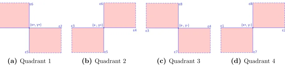
interval (uF −δ, uF +δ)∈ UF and (uG−δ, uG+δ)∈ UG there is an εi ≥0 such that
F+−1((uF −δ, uF +δ))⊆(x+−ε1, x++ε2)⊆[0, d1] (2.12a)
F−−1((uF −δ, uF +δ))⊆(x−−ε3, x−+ε4)⊆[−d2,0] (2.12b)
G−+1((uG−δ, uG+δ))⊆(y+−ε5, y++ε6)⊆[0, d3] (2.12c)
G−−1((uG−δ, uG+δ))⊆(y−−ε7, y−+ε8)⊆[−d4,0] (2.12d)
Each of the bounded intervals in (2.12) translate directly into thex, y pairs we generated
in (2.11). We can consider what this means for the behavior of the curve on the plane about
a particular point in each quadrant for some fixed c∈R+.
(a) Quadrant 1 (b) Quadrant 2 (c) Quadrant 3 (d) Quadrant 4
Figure 2.1: A graphical representation of the bounded behavior of the curve over the plane about a point in each quadrant. For some δ-ball defined over UF and UG there must be some x, y pairs within the shaded regions.
For any δ-ball which contains points inUF and UG there exists εi×εj rectangles about a
point in each quadrant corresponding to the shaded regions in Figure 2.1 which must contain
somex, y pairs. Asδ→0 so too must each ε, but by the monotonicity and continuity of the mappings in (2.10) for anyδ >0 there must be some open interval aboutxandybounded by
εi andεj. Asx→0 in each quadrant the pairs must approach the y-axis and asy→0 they
must approach the x-axis. As x →0 in quadrants one and two both paths converge to the same point on the positive y-axis at its maximum value, (0, d3), and similary for every other
and finite if and only ifc <∞. This path only passes through the origin if x=y = 0 which can occur if and only ifc= 0. All other paths must move about the origin.
Lemma 2. The generalized ellipse (2.1) expands and contracts continuously over the plane
with respect to c.
We will adopt much of the argumentative structure of Lemma 1. To expand or contract
the generalized ellipse we must change the value of the constant c. Consider a δ-ball about
a pointuF ∈ UF anduG ∈ UG such that for any change in cthere is an appropiate change in
uF and uG. If we add or subtract some value to cwe must add or subtract a value to both
uF and uG, instead of adding to one and subtracting from the other as in Lemma 1, such
that we maintain a summation to the new constant.
Suppose we add some amount δ >0 to c. For some arbitrary c >0 we can define a set
δ = [0, δ] ⊂ R+ such that there is a one to one and onto mapping between δ and U
F, and
δ and UG. This mapping will sum elements of each set in order so the relation in (2.1) is
satisfied such that
uF +δ1+uG+δ2 =c+δ (2.13)
for some δ1, δ2 ∈δ which sums toδ1+δ2 =δ, and similarly for subtraction.
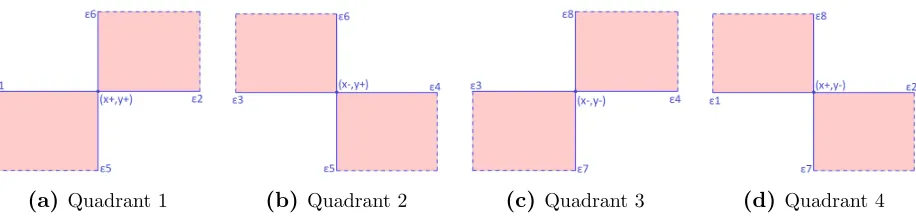
For any such c and δ there is always some ε > 0 such that there are εi ×εj rectangles
about a point in each quadrant which contain some x, y pairs, but because we are adding
to, or subtracting from, both uF and uG rather than adding to one and subtracting from
the other the εi×εj rectangles will now appear in the areas of expansion about the point
in each quadrant which were empty in Figure 2.1 — i.e., expansion and contraction of the
generalized ellipse occurs in a transverse direction to the circumference as shown in Figure
2.2. If the x, y point sits on an axis then the ε orthogonal to that axis is zero and the point
(a) Quadrant 1 (b) Quadrant 2 (c) Quadrant 3 (d) Quadrant 4
Figure 2.2: A graphical representation of the bounded behavior of the expansion and contraction of the curve over the plane about a point in each quadrant.
For any −∞< x <+∞on the plane such that F(x) =c1 <∞ and any−∞< y <+∞
on the plane such that G(y) = c2 <∞ there exists some c∈ R+ such that c1+c2 = c. So,
every point inR2 is in (2.6). For some fixedcthe generalized ellipse forms a continuous path
about the origin, each x and y value on this path appears uniquely in each quadrant, and
the generalized ellipse expands and contracts transversely to its path for all c∈R+. Thus,
each point (x, y) appears uniquely in (2.6).
2.2
Distance
Space has a very broad definition in mathematics, often simply defined as — a set with some
additional structure. We can use the generalized ellipses to provide this additional structure
over the plane.
Let us consider the generalized ellipse with the constant on the right hand side defined
by some function H : [0,∞) → [0,∞) such that it is strictly monotone, zero at the origin, and H → ∞ if and only if d→ ∞.
F(x) +G(y) =H(d) (2.14)
whereH(d) = c∈R+. This construction is similar to the generalized ellipse in (2.1), except
rather than fixing the constant and using this to define a set ofxand ywe will be providing
define the distance between two such points as
d(ai,aj) = H−1(F(xj−xi) +G(yj −yi)) (2.15)
A metric is frequently referred to in the literature as a distance function. We wish to
explore under what conditions metrics and other types of spaces can be formed by a particular
generalized ellipse, so we will refer to (2.15) as the distance function but this is not meant
to imply that it defines a metric. We will use (2.15) to explore the conditions on F, G, and
H necessary to generate a space with whatever particular properties we desire.
For some distance function over the plane there are four basic conditions which must be
satisfied to qualify as a metric:
1. d(ai,aj)≥0
2. d(ai,aj) = 0 ⇐⇒ ai =aj
3. d(ai,aj) =d(aj,ai)
4. d(ai,ak)≤d(ai,aj) +d(aj,ak)
The last three conditions are usually sufficient for defining a metric because they imply the
first condition.
Conditions 1 and 2 are implied by the construction of the generalized ellipse in
canon-ical position. A distance over a space which satisfies these first two conditions is called a
premetric. The last two conditions will require some constraints onF, G, and H.
Proposition 3. If both F and G are even, then (2.15) defines a semimetric.
Condition 3 requires that the distance necessary to go from a point a1 to a point a2 is
the same distance to go from a2 toa1. Proposition 2 establishes the conditions for F and G
under which there may be a guaranteed symmetry about the axes. This suggests requiring
and sufficient for satisfying condition 3. If Conditions 1,2, and 3 are satisfied, then (2.15) is
referred to as a semimetric in the literature.
Proposition 4. There exists an H such that (2.15) satisfies the triangle inequality.
The necessary conditions for satisfying this are far less apparent than the first three.
While the exact forms each of F,G, and H which satisfy subadditivity are not individually
obvious, we might loosely say that it is necessary for H to be linear or superlinear and its
initial order should be at least as large as or larger than that of F and G. This is a very
vague statement, so lets review some conditions of the triangle inequality to get a better
grasp of this concept.
The monotonicity of F, G, and H have several implications for subadditivity. Let’s
assume these functions are even. If|x3−x2|,|x2−x1|<|x3−x1|thenF(x3−x2), F(x2−x1)<
F(x3−x1) and similarly for the arguments of GandH. If it is not even then we would have
to handle the positive and negative arguments ofF,G, andH seperately, but it is not overly
that important we make this distinction now. Our concern will be with how the monotonic
behaviors ofF,G, andH interact to produce subadditivity. If|x3−x2|,|x2−x1|>|x3−x1|
then subadditivity is likely satisfied for those values. The more difficult case is when the
arguments for the functions on the right are less than the ones on the left and how they might
still sum to a greater distance. To that aim we introduce a simplification of notation which
is not meant to replace the lengths between points, but to make reviewing the interactions of
the function behavior more tractable. We will define the lengthsx3−x1 =x andy3−y1 =y
and we will assume that the point a2 lies between a1 and a3 such that x1 < x2 < x3 and
y1 < y2 < y3. We can then define an α, β ∈[0,1] such thatx2−x1 =αx, x3−x2 = (1−α)x,
y2−y1 =βy, and y3−y2 = (1−β)y. For some F, G, and H the triangle inequality must
satisfy
The essence of what the triangle inequality asks on the plane is if the direct distance
froma1 toa3 is the shortest way to get toa3, or can we pass through some point a2 on our
way to a3 which is shorter.
Define,
D=F(x) +G(y), D1 =F(αx) +G(βy), and D2 =F((1−α)x) +G((1−β)y) (2.17)
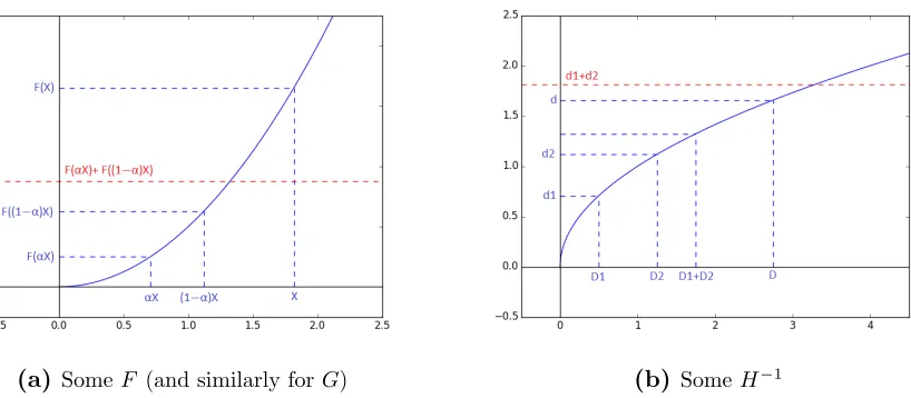
(a) SomeF (and similarly forG) (b) SomeH−1
Figure 2.3: Figure 2.3a plots a high growthF(x) and Figure 2.3b plots the inverse ofH. Each of these plots show the effect of the growth of the curve on the values used in the distance function (2.16).
Because the continuous functions F, G, and H are bounded for any finite values, even
though Figure 2.3a suggest that F and G may have a very high growth rate such that
F(x) +G(y)>> F(αx) +G(βy), F((1−α)x) +G((1−β)y) (2.18)
Figure 2.3b suggests there exists an H which can be chosen as a crude blugeon to force
(2.16) to satisfy subadditivity. We merely need some H whose inverse has a rapid initial
growth rate, which then continually decreases similar to Figure 2.3b, such that the sum of
the resultants of the two smaller arguments have sufficient size to be larger than the resultant