University of New Orleans University of New Orleans
ScholarWorks@UNO
ScholarWorks@UNO
University of New Orleans Theses and
Dissertations Dissertations and Theses
Spring 5-15-2015
Three-Dimensional Ideal Gas Reference State based Energy
Three-Dimensional Ideal Gas Reference State based Energy
Function
Function
Avdesh Mishra
University of New Orleans, [email protected]
Follow this and additional works at: https://scholarworks.uno.edu/td
Part of the Biochemical and Biomolecular Engineering Commons, Biochemistry Commons, Bioinformatics Commons, Biophysics Commons, Computational Engineering Commons, Molecular Biology Commons, and the Structural Biology Commons
Recommended Citation Recommended Citation
Mishra, Avdesh, "Three-Dimensional Ideal Gas Reference State based Energy Function" (2015). University of New Orleans Theses and Dissertations. 1986.
https://scholarworks.uno.edu/td/1986
This Thesis is protected by copyright and/or related rights. It has been brought to you by ScholarWorks@UNO with permission from the rights-holder(s). You are free to use this Thesis in any way that is permitted by the copyright and related rights legislation that applies to your use. For other uses you need to obtain permission from the rights-holder(s) directly, unless additional rights are indicated by a Creative Commons license in the record and/or on the work itself.
Three-Dimensional Ideal Gas Reference State based Energy Function
A Thesis
Submitted to the Graduate Faculty of the University of New Orleans In partial fulfillment of the Requirements for the degree of
Master of Science in
Computer Science
by
Avdesh Mishra
BS in Computer Engineering, Tribhuvan University, 2012
ii
Table of Contents
List of Figures ... iii
List of Tables ...iv
ABSTRACT ... v
INTRODUCTION ... 1
MATERIALS and METHODS ... 3
Residue Specific All-Atom Probability Discriminatory Function based Potential... 3
DFIRE Based Potential ... 6
3DIGARS, the Proposed Approach ... 8
GA over Grid Search for Optimal Parameter ... 13
DATASET COLLECTION and DECOY DATASETS ... 14
Training Dataset ... 14
Decoy Datasets ... 16
Moulder Decoy-set ... 17
Rosetta Decoy-set ... 17
I-Tasser Decoy-set-II ... 17
4state_reduced ... 18
Fisa ... 18
Fisa_casp3 ... 18
Hg_structal ... 18
Ig_structal ... 18
Ig_structal_hires ... 19
Lattice_ssfit ... 19
Lmds ... 19
RESULTS ... 19
CONCLUSIONS ... 22
SUPPLEMENTARY CONTENT ... 23
REFERENCES ... 23
iii
List of Figures
FIGURE 1:(A)NATIVE LIKE PROTEIN CONFORMATION 25, PRESENTED IN A 3D HEXAGONAL-CLOSE-PACKING (HCP)
CONFIGURATION USING HYDROPHOBIC (H) AND HYDROPHILIC OR POLAR (P) RESIDUES.THE H-H INTERACTIONS SPACE IS RELATIVELY SMALLER THAN P-P INTERACTIONS SPACE, SINCE HYDROPHOBIC RESIDUES (BLACK BALL)
BEING AFRAID OF WATER TENDS TO REMAIN INSIDE OF THE CENTRAL SPACE.(B)3D METAPHORIC HP FOLDING KERNELS, DEPICTED BASED ON HCP CONFIGURATION BASED HP MODEL, SHOWING THE 3 LAYERS OF
DISTRIBUTIONS OF AMINO-ACIDS 25,26. ... 3
FIGURE 2:FITNESS VERSUS Α_HP,Α_HH AND Α_PP VALUES.THE VALUES REMAIN STABLE DURING OPTIMIZATION,
iv
List of Tables
TABLE 1:HYDROPHOBIC (H)/HYDROPHILIC (P) CATEGORIZATION OF THE AMINO ACIDS. ... 10
TABLE 2:PERFORMANCE OF TWO DIFFERENT REFERENCE STATE ON TRAINING DATASET DIFFERED BY MAXIMUM RESOLUTION AND SIMILARITY CUTOFF WHILE KEEPING OTHER PARAMETERS SUCH AS EXPERIMENTAL METHOD AS
“IGNORE”, MOLECULE TYPE AS “PROTEIN”, REFINEMENT R-FREE OF MINIMUM 0.0 AND MAXIMUM 0.25, NUMBER OF CHAINS AS “SINGLE CHAIN” IF NOT MENTIONED. ... 20
TABLE 3:COMPARISON BETWEEN DFIRE,RWPLUS, DDFIRE,DFIRE2.0 AND OUR ENERGY FUNCTION (3DIGARS) ON 11 DECOY SETS BASED ON CORRECT SELECTION OF NATIVE FROM THEIR DECOY SET AND Z-SCORE. ... 21
v
ABSTRACT
Energy functions are found to be a key of protein structure prediction. In this work, we propose a novel
3-dimensional energy function based on hydrophobic-hydrophilic properties of amino acid where we
consider at least three different possible interaction of amino acid in a 3-dimensional sphere categorized
as hydrophilic versus hydrophilic, hydrophobic versus hydrophobic and hydrophobic versus hydrophilic.
Each of these interactions are governed by a 3-dimensional parameter alpha used to model the interaction
and 3-dimensional parameter beta used to model weight of contribution. We use Genetic Algorithm (GA)
to optimize the value of alpha, beta and Z-score. We obtain three energy scores libraries from a database
of 4332 protein structures obtained from Protein Data Bank (PDB) server. Proposed energy function is
found to outperform nearest competitor by 40.9% for the most challenging Rosetta decoy as well as better
in terms of the Z-score based on Moulder and Rosetta decoy sets.
1
INTRODUCTION
History of protein structure prediction is based on the thermodynamic hypothesis that the native
structure gains the lowest free energy compared to the other decoys or the intermediate
conformations under same physiological conditions 1. A decent potential that can discriminate
between native and nearly infinite number of possible decoy structures is vital for protein
structure prediction. So far many attempts have been made towards development of better energy
function which can be categorized into two different types 2; 3; 4; 5; 6 i) physical-based potential,
based on molecular dynamics or computation of atom-atom forces 7; 8; and ii) knowledge-based
potentials, obtained from statistical analysis of known protein structure 9; 10; 11; 12; 13; 14. Some of
the energy functions are modelled based on only backbone alpha carbon atom whereas, many of
these are based on all atom (167 heavy atoms), knowledge based, distance dependent potential.
They vary from one another based on the reference state and the type of physical features they
employ to counterbalance sampling bias 15. For example, Kortemme et al. 16 obtained a
knowledge-based hydrogen-bonding potential. Yang and Zhou incorporated polar-polar and
polar-nonpolar orientation dependence to the distance-dependent knowledge-based potential
based on a distance-scaled, finite-ideal gas reference (DFIRE) state 17 by treating polar atoms as
a dipole (dDFIRE) 18. Lu et al. 19 defined side-chain orientation according to rigid blocks of
atoms (OPUS-PSP). Zhang and Zhang 20 employed orientation angles between two vector pairs
predefined for each side-chain (RWplus). Zhou and Skolnick improved over the DFIRE energy
function by incorporating relative orientation of the planes associated with each heavy atom
(GOAP) 21. For obvious reasons, the relatively complete and detail approaches are the all atom
based approaches. The efficacy of the all-atom based approach relay heavily on the formulation
2
well as knowledge based approach that derives an effective energy function from known protein
structures with multidimensional reference states.
We propose an improved potential based on four factors i) better training dataset; ii) three
different energy scores based on hydrophobic and hydrophilic categorization of residue-atom
pairs; iii) three different alpha values for three different energy scores generation; and iv) three
different weights of contribution of energy scores. Fundamental work of DFIRE considers
residues placed in a modified spherical environment controlled by the single dimensional
parameter (alpha), where the alpha value is used to calculate the volume of the sphere
considering the spherical environment as a finite system 10. On the contrary, our motivation
towards this work comes from the fact that – amino acids, based on their types are not distributed
equally over the 3D structure of a protein to consider them in the same scale on an average by a
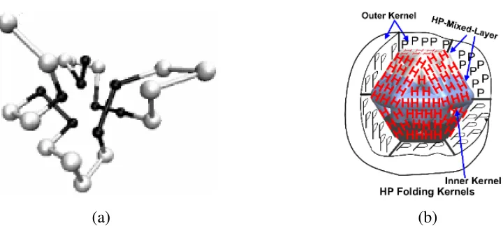
single dimensional parameter (see Fig. 1(a)). Rather they can be segregated into at least 3
different categories based on the usual distribution with the protein conformations (see Fig.
1(b)). Related to this, hydrophobic-hydrophilic or hydrophobic-polar (HP) model considers
hydrophobic (H) amino acids having fear of solvent like water, they want to keep themselves
away from aqueous solvent forming the core or inner-kernel 22 of protein and thus remain inside
of a protein. On the other hand, the hydrophilic or the polar (P) amino acid or residues being
attracted to water, try to remain outside the core, forming the outer-kernel (see Fig. 1 (b)). Thus
Ps are often found on the outside of their folded structure 23; 24, and in between this two layer
there is a thin HP-mixed-layer 22. Following these aforementioned properties, we proposed our
multidimensional reference states based energy function 3DIGARS (3 Dimensional Ideal Gas
3
(a) (b)
Figure 1: (a) Native like protein conformation 25, presented in a 3D hexagonal-close-packing (HCP) configuration
using hydrophobic (H) and hydrophilic or polar (P) residues. The H-H interactions space is relatively smaller than P-P interactions space, since hydrophobic residues (black ball) being afraid of water tends to remain inside of the central space. (b) 3D metaphoric HP folding kernels, depicted based on HCP configuration based HP model, showing the 3 layers of distributions of amino-acids 25, 26.
The remainder of this paper proceeds as follows. We review the evolution of the relevant
theories and underpinning theoretical aspect of our proposed approaches in Section 2. Section 3
discusses our approach for training data collections as well as the collections of the
decoy-datasets to be used for measuring performances of our approach compared to other
state-of-art-approaches. We discussed the obtained results in Section 4 and finally Section 5 concludes the
proposed energy function.
MATERIALS and METHODS
Residue Specific All-Atom Probability Discriminatory Function based
Potential
Initially, the residue specific all-atom probability discriminatory function (RAPDF) based energy
function was proposed by Samudrala and Moult 9 which was based on averaging reference state.
In this approach, the energy score of a conformation was computed in two different ways:
conditional probability based approach and free energy based approach. It was found that these
two approaches are equivalent for all practical purposes while it is more easier to work with
4
aspect of it: an equilibrium distribution of atom pairs, the physical nature of the reference state
and the probability of observing a system in any given state which is also subject to change with
respect to the temperature 2.
Conditional probabilities of pairwise atom-atom interactions in proteins can be computed
using statistical observation of native structures 9 from protein-databases such as Protein Data
Bank 27. The conditional probabilities are based on two different type of structures one which is
native (N) and the other is the near native or decoy (D). Energy potentials are developed based
on the pairwise atom-atom interactions of native structures. Pairwise atom-atom distance is a set
of intra-atomic separation within a structure represented as { ij}
ab
S , where {Sabij} is the distance
between atom i and j of amino acid type a and b, respectively. The probability that the atom pairs
separated by distance { ij}
ab
S belongs to native conformation can be represented by P(N|Sabij ).
Therefore, we can write the general formula of conditional probability that, atom pairs separated
by distance { ij}
ab
S belongs to native conformation as:
) ( / )) ( * ) | ( ( ) | ( ij ab ij ab ij
ab P S N P N P S
S N
P = (1)
Assuming that all distances are independent of each other, conditional probabilities can be
expressed as the probabilities of observing the set of distances as products of the probabilities of
observing each individual distance 9
∏
= ij ij ab ijab N P S N
S
P( | ) ( | ) and =
∏
ij ij ab ij
ab P S
S
P( ) ( ) (2)
Substituting the Eq. 1 by Eq. 2 we get Eq. 3:
∏
= ij ij ab ij ab ijab P N P S N P S
S N
5 )
(N
P in above equation is a constant and independent of conformation of given structure and so
it can be omitted from further consideration. Omission of P(N) implicates that scores from
different sequences cannot be compared. Thus the log form of Eq. 3 is used to both scale the
quantities to a small range and to give a form similar to that of potential of mean force. Scoring
function SF proportional to the negative log conditional probability that the structure is correct
can be written as:
(
|{ })
ln ) ( / ) | ( ln })
({ ij
ab ij
ij ab ij
ab ij
ab P S N P S K P N S
S
SF = −
∑
− (4)Therefore, given a protein structure or conformation, using Eq. 4, we can calculate all the
distance separation between all pairs of atom types and compute the total energy by summing up
the probability ratios assigned to each separation between a pair of atom types. Thus, we can
compute the probability of observing atom type a and b in a particular bin which is S distance
apart in a native conformation P(Sab|N) as:
∑
=
s
ab ab
ab N N S N S
S
P( | ) ( )/ ( ) (5)
where N(Sab) is the frequency of observation of atom type a and b in a particular bin which is of
S distance apart. The denominator is the number of such observation for all bins.
The denominator in Eq. 5 is the average over different atom types in the experimental
conformations which represents the random reference state. Thus the probability of seeing any
two atom types a and b in a bin which is S distance apart can be represented as:
∑
∑∑
=
ab S ab
ab ab
ab N S N S
S
6
where,
∑
ab ab
S
N( ) is the total number of counts summed over all pairs of atom types in a
particular distance S, and the denominator is the total number of counts summed over all pairs of
atom types summed over all bins.
As RAPDF energy function is based on averaging reference state, it does not consider the
distribution of amino acid in 3D conformational space whereas DFIRE based potential considers
protein as a sphere comprising of uniformly distributed atoms and also suggest that the radius of
such spheres does not increase in 2
r as in an infinite system rather protein is a finite system and
so the increase in the radius is represented by α (a variable which can be ≤ 2). This involved our
concerns toward more detailed study into DFIRE based potential.
DFIRE Based Potential
Distance-scaled, finite ideal-gas reference (DFIRE) state is a distance-dependent, all atom,
knowledge-based potential 10. The reference state formulation in DFIRE is more appealing and
effective over RAPDF. The reference state RAPDF uses an averaged distribution over all residue
or atom pairs whereas, DFIRE uses pair distribution function from statistical mechanics to
formulate finite ideal-gas reference state.
The basis of finite ideal-gas reference state can be explained by exploring the
fundamental equation of statistical mechanics for infinite system. For an infinite system the
observed number of pairs of atoms, namely th
i and jth atoms, denoted as Nobs(i,j,d), at spatial
distance d with tolerance ±∆d is related to the pair distribution function gij(d), which describes
how density varies as a function of distance from a reference particle and can be represented as:
) 4
)( ( 1
) , ,
( 2
d d d g N N v d j i
N ij
s j s i s
obs = π ∆
7
where volume of the system is represented as s
v , Nis and s j
N are the number of th
i and jth
atoms in a system, respectively. The potential based on pairwise distance P(i, j,d) can be
written as: ))) 4 ( /( ) * ) , , ( ln(( ) , , ( 2 d d N N V d j i N RT d j i
P =− obs s is sj π ∆ (8)
In case there is no interaction between the atoms, we can write: P(i, j,d) = 0, thus from Eq. 8
we can have:
) / 4 ( ) , , ( ) , , ( 2
exp sj s
s i
obs i j d N N d d v
N d j i
N = = π ∆ (9)
Equations above from statistical mechanics can directly be applied in infinite system whereas the
proteins are finite system, therefore, the pair density will not increase by square factor (i.e., 2
d ),
rather it increase by some factor α (i.e., dα ) which was determined by the best fit of dα
considering number of points in 1011 finite protein size spheres.
Thus, Eq. 9 can be written as:
) / 4 ( ) , , (
exp sj s
s
i N d d v
N d j i
N = π α∆ (10)
Further, Eq. 8 can be rewritten as:
))) 4 ( /( ) * ) , , ( ln(( ) , ,
(i j d RT N i j d V N N d d
P =− obs s is sj π α∆ (11)
Assuming that there is no interaction beyond cutoff distance of dcut or P(i, j,d) = 0 at d≥ dcut,
d is replaced by dcut. This leads Eq. 11 to form Eq. 12:
) , , ( ) , , ( ln ) , , ( cut obs cut cut obs d j i N d d d d d j i N RT d j i P ∆ ∆ −
8
Here, a constant η is placed for mutation induced changes and is also needed because
temperature is a free parameter in potentials derived from static structures. Eq. 12 implies new
equation for Nexp(i,j,d):
) , , ( ) , , (
exp obs cut
cut cut d j i N d d d d d j i N ∆ ∆ = α (13)
It is to be noted that the Eq. 13 does not contains any distance dependent term rather it is a
formulation obtained from ideal gas reference state implementable for finite system.
Similar to the approaches in Samudrala and Moult 9, DFIRE also uses 167 heavy atom
types. The cutoff distance dcut is = 14.5 Å. The bin width ∆d have different width for d < 2 Å,
∆d=2 Å, for 2 Å < d < 8 Å, ∆d=0.5 Å and for 8 Å < d < 15 Å, ∆d=1 Å. Thus, the total number of
bins is 20. Bin width and dcut were not optimized.
3DIGARS, the Proposed Approach
Based on the hydrophobic-hydrophilic model (HP model) we constructed three different energy
score libraries with bin size, ∆r = 0.5 Å each, with a cutoff distance of 15 Å, where r represents
each distant bin with values ranging from 0.5 Å to 15 Å. The value of cutoff bin ∆rcut = 0.5 Å as
all bin size are same. Residue-atom pairs within same residue were ignored while constructing
energy score libraries. We name these libraries as i) hydrophobic-hydrophilic (HP); ii)
hydrophobic-hydrophobic (HH); and iii) hydrophilic-hydrophilic (PP) interactions libraries and
each of these libraries comprises of its independent reference state. Reference state
corresponding to hydrophobic-hydrophilic group can be written as:
)) , , ( ) , , ( ) , , ( ( ) (
, obs HP cut obs HH cut obs PP cut
cut cut
HP EXP
j
i N i j r N i j r N i j r
9
where NiEXP,j −HP(r) represents the expected number of atom pairs at distance r for hydrophobic
versus hydrophilic interaction, Nobs−HP(i,j,rcut) represents observed number of atom pairs th
i and
th
j at cutoff distance in hydrophobic-hydrophilic library, Nobs−HH(i,j,rcut) represents observed
number of atom pairs th
i and jth at cutoff distance in hydrophobic-hydrophobic library,
) , ,
( cut
PP
obs i j r
N − represents observed number of atom pairs th
i and jth at cutoff distance from
hydrophilic-hydrophilic library and αhp is the parameter that belongs to hydrophobic versus
hydrophilic group which is obtained by GA.
Similarly, reference state corresponding to hydrophobic-hydrophobic group can be written as:
)) , , ( ) , , ( ) , , ( ( ) (
, obs HP cut obs HH cut obs PP cut
cut cut
HH EXP
j
i N i j r N i j r N i j r
r r r r r N hh − − − − + + ∆ ∆ = α (15)
where NiEXP,j −HH(r) represents the expected number of atom pairs at distance r for hydrophobic
versus hydrophobic interaction, αhh is the parameter that belongs to hydrophobic versus
hydrophobic group which is also obtained by GA and rest of the terms are as defined under Eq.
14.
Finally, reference state corresponding to hydrophilic-hydrophilic group can be written as:
)) , , ( ) , , ( ) , , ( ( ) (
, obs HP cut obs HH cut obs PP cut
cut cut
PP EXP
j
i N i j r N i j r N i j r
r r r r r N pp − − − − + + ∆ ∆ = α (16)
where NiEXP,j −PP(r) represents the expected number of atom pairs at distance r for hydrophilic
versus hydrophilic group, αpp is the parameter that belongs to hydrophilic-hydrophilic group
10
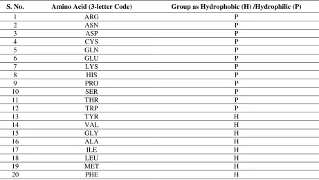
While generating energy score libraries, residue-atom pairs are categorized to identify which of
the group (HP, HH or PP) mentioned above they fall in e.g. while considering interaction
between two Nitrogen (N) atom of amino acid Alanine (ALA:N versus ALA:N), we categorize
this interaction as hydrophobic-hydrophobic (HH) group as amino acid ALA (Alanine) is
hydrophobic in nature. Similarly, while considering interaction between Nitrogen (N) atom of
amino acid Arginine (ARG) and Carbon (C) atom of amino acid Serine (SER); (ARG:N versus
SER:C), we categorize this interaction as hydrophilic-hydrophilic (PP) as both residues Arginine
(ARG) and Serine (SER) are hydrophilic in nature. The categorization of amino acid into
hydrophobic and hydrophilic group is obtained from 24 also shown in Table 1.
Table 1: Hydrophobic (H)/ Hydrophilic (P) categorization of the amino acids.
S. No. Amino Acid (3-letter Code) Group as Hydrophobic (H) /Hydrophilic (P)
1 ARG P
2 ASN P
3 ASP P
4 CYS P
5 GLN P
6 GLU P
7 LYS P
8 HIS P
9 PRO P
10 SER P
11 THR P
12 TRP P
13 TYR H
14 VAL H
15 GLY H
16 ALA H
17 ILE H
18 LEU H
19 MET H
20 PHE H
Along with the categorization of residue-atom pairs the frequency counts of the specific
group is updated simultaneously. Further these energy score libraries are used for total energy or
minimum energy calculation. Once we compute frequencies of all the 3 groups, we generate
11 )) ( / ) , , ( ln( , ,
, N i j r N r
ESiHPjr =− obs−HP iEXPj −HP (17)
where HP
r j i
ES,, is the energy score of atom pair ith and jth at distant bin r for group HP,
) , , (i j r
Nobs−HP is the observed number of atom pair th
i and jth at distant bin r for HP group and
) (
, r
NiEXPj −HP is expected number of atom pairs at distance r for HP group as defined in Eq. 14.
Similarly energy score for HH group can be written as:
)) ( / ) , , ( ln( , ,
, N i j r N r
ESiHHjr =− obs−HH iEXPj −HH (18)
where HH
r j i
ES,, is the energy score of atom pair th
i and
j
th at distant bin r for group HH,)
,
,
(
i
j
r
N
obs−HH is the observed number of atom pair thi and
j
th at distant bin r for HH group and) (
, r
NiEXPj HH
−
is expected number of atom pairs at distance r for HH group as defined in Eq. 15.
Finally energy score for PP group can be written as:
)) ( / ) , , ( ln( , ,
, N i j r N r
ES obs PP iEXPj PP
PP r j i − − − = (19)
where PP
r j i
ES, , is the energy score of atom pair ith and
th
j
at distant bin r for group PP,)
,
,
(
i
j
r
N
obs−PP is the observed number of atom pair ith and thj
at distant bin r for PP group and) (
, r
NiEXPj −PP is expected number of atom pairs at distance r for PP group as defined in Eq. 16.
Later minimum energy or total energy of decoy set as well as native proteins are
calculated from these energy score libraries. We use weight factors βhp, βhh, and βpp to
optimize the contribution of each of the three energy score libraries. So, total energy (TE) of the
protein conformation can be written as:
pp pp hh hh hp
hpE E E
12
where βhp, βhh, and βpp are 3D weights of contribution and Ehp, Ehh, and Epp are the energy
scores obtained from three groups HP, HH and PP. Here Ehp can be written as:
∑
= r j i HP r j i hp ES E , , , , (21)Similarly, Ehh can be written as:
∑
= r j i HH r j i hh ES E , , , , (22)And, Epp can be written as:
∑
= r j i PP r j i pp ES E , , , , (23)We use Genetic Algorithm (GA) for determining the best possible values of alpha (αhp,
hh
α and
pp
α ), and optimized the contributions of each of the three group by determining their
appropriate weights βhp, βhh, and βpp along with the z-score to discriminate the native from
their decoys, where z-score of native structure is defined as:
SD average native E E E
Z = − (24)
where Enative is the energy of native protein, Eaverage is the average energy of decoy sets
corresponding to the same protein excluding native protein itself and ESD is the standard
deviation of the energies of all the decoy sets corresponding to the same protein.
In the optimization using GA, the value of alpha and beta ranges from 0 to 2 and -2 to 2
respectively. GA parameters were set as i) population size of 50, ii) single-point crossover and
mutation, iii) elite rate of 5%, iv) crossover rate of 90% and v) mutation rate of 50%. Scores
13
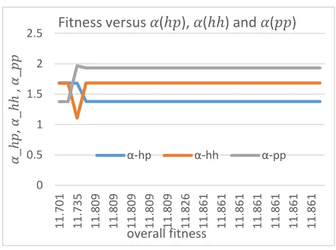
Figure 2: Fitness versus α_hp, α_hh and α_pp values. The values remain stable during optimization, ensure
reliabilities.
The obtained best values of alphas are: αhp= 1.3802541, αhh = 1.6832844 and
pp
α =
1.9315737. The obtained best beta values are βhp= 1.4921875, βhh= 0.55859375 and βpp=
0.265625. Plot of obtained fitness versus αhp, αhh and
pp
α values at each generation in Fig.2
shows the GA performance on selecting best fitness and also consistency of obtained fitness with
values of αhp, αhh and αpp.
GA over Grid Search for Optimal Parameter
In context of this application, search for optimal parameter involves i) generating 3D
energy score libraries each time for 3D alpha values and ii) computing correct count and z-score
of three decoy sets Moulder, Rosetta and Tasser each time for 3D beta values. Our goal is to
obtain the best value of 3D alpha and 3D beta which provides us the maximum correct count for
each of the decoy sets and high negative z-score. Generating 3D energy score libraries involve
processing of 4332 native protein structures residing in hard drive. In addition, computing
correct count and z-score of three decoy sets Moulder, Rosetta and Tasser involves processing of
20, 58 and 56 proteins respectively. Each of these proteins have around 600 decoy files on an 0 0.5 1 1.5 2 2.5 1 1 .7 0 1 1 1 .7 3 5 1 1 .8 0 9 1 1 .8 0 9 1 1 .8 0 9 1 1 .8 0 9 1 1 .8 0 9 1 1 .8 2 6 1 1 .8 6 1 1 1 .8 6 1 1 1 .8 6 1 1 1 .8 6 1 1 1 .8 6 1 1 1 .8 6 1 1 1 .8 6 1 ߙ _ ℎ , ߙ _ ℎ ℎ , ߙ _ overall fitness
Fitness versus ߙ(ℎ), ߙ(ℎℎ) and ߙ()
14
average and so, on an average we need to process 80,400 files. Thus, on each iteration we need
to process 84,732 structure files.
Furthermore, our application involves obtaining optimal parameter for 3D alpha values as
well as 3D beta values, totaling to 6 variables needed to be optimized. We choose GA to tackle
this search problem involving multiple variables and huge I/O (Input/Output) operation over
Grid Search because, GA searches for the global optima and converses quickly or in other words
provides the results in few steps as shown in Fig. 2 whereas, Grid Search involves nested loop
search. As our search space involves 3D alpha and 3D beta variables ranging from 0 to 2 and -2
to 2 respectively the Grid Search based approach involves 6 nested loops and each iteration
involves huge I/O operations. In addition, Grid Search involves step size which is of greater
importance, if we select a step size of greater width there exist a possibility of missing the
optimal value whereas, if we use a finer grid search (small step size such as 0.01) we might end
up running the process for months. Thus to obtain better result in considerable amount of time
we selected GA over Grid Search based approach for optimal parameter search.
To access the performance of our 3DIGARS energy function we tested it with most
challenging decoy sets as well as moderately challenging decoy sets in Table 3 against the state
of art approaches DFIRE, RWplus, dDFIRE and DFIRE2.0 based on the number of correctly
identified proteins and average z-score for three different decoy sets.
DATASET COLLECTION and DECOY DATASETS
Training Dataset
Datasets to generate energy score were obtained from three different sources, PDB (Protein Data
Bank) server, ccPDB 28 (Compilation and Creation of datasets from PDB) server and PISCES 29
15
obtained from all experimental method, structures better than 1.5 Å resolution, R-factor of 0.0 to
0.25, chain length 40 or more and less than or equal to 30% sequence identity cutoff from all the
three sources mentioned above.
Performance of these long multiple chain sequence datasets were very poor which lead us
to exhaustively generate many different datasets with different specifications. Poor results from
multiple and long chain dataset lead us towards some research for less number of chains and
shorter chain length sequences. We generated dataset with number of chain 0 to 2 with maximum
chain length of 1000, results from this specification was similar to the result obtained from
multiple and long chain sequences. Later we collected dataset with minimum resolution 0.0 and
maximum resolution 1.5, similarity cutoff 30%, single chain and maximum chain length of 500.
This single chain and shorter length protein sequences gave us comparably better result than
multiple chain. Thus we focused our research on single chain proteins. As we moved from
multiple chain sequences to single chain we continued working only with PDB dataset because,
we were unable to collect only single chain sequences from PISCES and ccPDB servers.
We exhaustively generated many single chain datasets with different specifications. To
generate dataset less than or equal to 25% sequence identity we used a sequence clustering
program BLASTCLUST 30. While executing BLASTCLUST we found that it fails if the
sequence length is less than 7 reside long and if the sequences have “X” or “U” (unknown
residue) in a sequence. Additionally, it fails if there are more than 4 protein id’s with different
chain id’s (>10jh_A, >10jh_B, >10jh_C, >10jh_D, >10jh_E and so on) in a FASTA input file. It
also fails if four or more sequences are exactly same. To overcome BLASTCLUST problems we
have an in-house program to remove the sequences that are shorter (< 7 residues) and also
16
Furthermore, we also wrote a program which removes proteins with missing residues in
the middle of the protein sequence. However, the program does not ignore the sequence if it has
missing residues at terminals (5 residues from each end). Thus our final training dataset consist
of only single chain protein sequences which are purified not to contain any proteins consisting
of missing residues anywhere except the terminal regions. We generated purified dataset keeping
all other specification common besides maximum resolution ranging from 1.5 to 2.5 and
sequence identities cutoff, of 25%, 30%, 40%, 50%, 70% and 100%. The best result overall of
these combination is obtained from collection of 4332 proteins from PDB which are single chain,
missing residue purified, has 100% sequence identity cutoff, minimum resolution of 0.0 and
maximum resolution of 2.5 and R-free of 0.25. This best collection before purification for
missing residues had 10602 proteins. The results obtained from 70% sequence identity cutoff is
very close to the result obtained from 100% sequence identity with later having slight
improvement. Selecting proteins with 100% identity cutoff mean we are actually preserving
actual representation of frequency distribution of amino acids in nature. This result suggest us
that the current PDB has huge collection of proteins now, which is sufficient to gives us proper
frequency distribution of the atom pairs in nature. Results obtained from all of the above
specifications are mentioned in Table 2.
Decoy Datasets
Performance of 3DIGARS was evaluated on 11 different decoy datasets which are described in
brief below. Three decoy sets Moulder, Rosetta and Tasser among the set of 11 decoys are
17
Moulder Decoy-set
Moulder 31 decoy set consist of 20 proteins for which 300 comparative models were built using
homologous template. The models were build using alignment that did not shared more than
95% of identically aligned positions or had at least 5 different alignment positions. These decoys
were build using MODELLER-6 program which applied default model building routine with
fastest refinement which keeps most of the template structure unchanged and are different from
decoys that are generated by ab initio folding that have all structure regions reassembled from
scratch.
Rosetta Decoy-set
Decoy set for 58 proteins were generated by Baker Lab which contains 20 random models and
100 lowest scoring models from 10,000 decoys using ROSETTA de novo structure prediction
followed by all-atom refinement 32. Current Rosetta decoy set has been improved than the
original Rosetta decoy set by adding side chains to the centroid/backbone models and refining
the structures to remove steric clashes. The improvement over original Rosetta were based on
four important points required to generate optimal decoy sets 1) decoy set should contain
conformations for a wide variety of different proteins to avoid over fitting; 2) decoy set should
contain conformation close to (< 4Å) to the native structure; 3) decoy set should consist of
conformations that are at least near local minima of energy potential; and 4) decoy set should be
produced without using information from native structure 33.
I-Tasser Decoy-set-II
I-Tasser 34 decoy set-II were generated first by using Monte Carlo Simulations and then refined
18
network 34. This set contains of 56 proteins each of which contains 300-500 decoys generated by
both template-based modeling and atomic-level structure refinement.
4state_reduced
This decoy set consist of 7 proteins. The CA positions for these decoys were generated by
choosing ten residues in each protein using a 4-state off-lattice model. All atom models were
built from the CA atoms with the program segmod 35.
Fisa
This set contains decoys for four small alpha-helical proteins. Main chains were generated using
a fragment insertion simulated annealing procedure [Simons et al] whereas side chains were
modelled with SCWRL package 36.
Fisa_casp3
This set contains 5 proteins. It contains decoys for proteins predicted by the Baker group for
CASP3. Main chain for these decoys were also generated using a fragment insertion simulated
annealing procedure whereas side chains were modelled with SCWRL package 36.
Hg_structal
This set contains decoys for 29 globins. Each proteins is built by comparative modelling using 29
other globins using 37.
Ig_structal
This set contains 61 immunoglobulins each of these is built by comparative modelling suing all
19
Ig_structal_hires
This set contains 20 immunoglobulins which is high resolution subset of immunoglobulins decoy
set. The resolution range for this set is 1.7-2.2 Å compared to full 61 set which has resolution
range from 1.7-3.1 Å. These sets are also build by comparative modeling using all other
immunoglobulins as templates using segmod program 37.
Lattice_ssfit
This set contains eight small proteins generated by ab initio methods 38.
Lmds
The local minima decoy set (lmds) contains of ten proteins derived from experimental secondary
structures of ten small proteins that belong to diverse structural classes. Two of the proteins were
CASP3 targets 39.
Decoy sets 4state_reduced, fisa, fisa_casp3, hg_structal, ig_structal, ig_structal_hires,
lattice_ssfit and lmds were obtained from http://dd.compbio.washington.edu/.
RESULTS
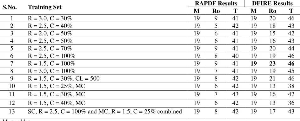
During our search for the best training dataset, we calculated the correct count of most
challenging decoy set by applying two different reference state to the collection of the dataset.
Table 2 implicates the exhaustive search of best dataset. The best correct count combination for
MOULDER, ROSETA, and TASSER was obtained from the training dataset with resolution 1.5
and sequence similarity 100% which is 19, 23, 46 respectively (see Table 2). This motivated us
to select the dataset with sequence similarity 100% and maximum resolution ranging from 1.5 to
20
From Table 2 we can also see that DFIRE based energy function outperforms RAPDF based
energy function which motivated us towards improvement over DFIRE based reference state.
Table 2: Performance of two different reference state on training dataset differed by maximum resolution and
similarity cutoff while keeping other parameters such as experimental method as “Ignore”, molecule type as “Protein”, refinement R-free of minimum 0.0 and maximum 0.25 , number of chains as “Single Chain” if not mentioned.
S.No. Training Set RAPDF Results DFIRE Results M Ro T M Ro T
1 R = 3.0, C = 30% 19 9 41 19 20 46
2 R = 2.5, C = 40% 19 5 42 19 18 43
3 R = 2.0, C = 50% 19 6 41 19 15 42
4 R = 2.5, C = 50% 19 6 41 19 16 43
5 R = 2.5, C = 70% 19 9 41 19 20 44
6 R = 2.5, C = 100% 19 8 40 19 19 46
7 R = 1.5, C = 100% 19 9 41 19 23 46
8 R = 3.0, C = 100% 19 7 41 19 19 45
9 R = 1.5, C = 30%, CL = 500 19 8 42 19 21 46 10 R = 1.5, C = 25%, MC 19 6 42 19 13 38 11 R = 1.5, C = 30%, MC 19 7 43 19 16 42 12 R = 1.5, C = 40%, MC 19 6 42 19 13 36 13 SC, R = 2.5, C = 100% and MC, R = 1.5, C = 25% combined 19 8 42 19 17 43
M- moulder Ro- rosetta T- tasser
R- maximum resolution C- similarity cutoff CL- chain length MC- multiple chain SC- single chain
Moulder Total Targets: 20, Rosetta Total Targets: 58, Tasser Total Targets: 56. DFIRE results are based on the DFIRE reference state with alpha = 1.57.
Furthermore, in Table 3 value within the parenthesis are average z-scores of the native
structures and values outside of parenthesis are number of correct count. Here the term correct
count can be described as the number of correctly identified native proteins from its decoy sets.
Good energy function is the one which can assign highest energy to the native proteins compared
to its decoy sets and thus is able to classify native proteins from its decoy sets more efficiently.
In other words correct count implicates that an efficient energy function can identify more native
21
dDFIRE are obtained from the GOAP: A Generalized Orientation-Dependent, All-Atom
Statistical Potential from Protein Structure Prediction 40. Correct count and z-score for DFIRE2.0
is computed from DFIRE2.0 package freely available from the Sparks Lab online server 41.
Correct counts by (3DIGARS) is calculated using energy score libraries generated using the
dataset with resolution 1.5, sequence similarity cutoff of 100%, keeping all other parameters
used for data collection common as described in DATASET section above. Table 3 clearly
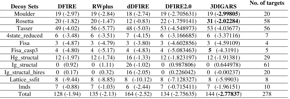
shows that hydrophobic and hydrophilic based energy function outperform DFIRE, RWplus,
dDFIRE and DFIRE2.0 based energy functions for most challenging Rosetta decoy-set and also
for decoy-set fisa_casp3. It is to be noted that RWplus computed 56 out of 56 for their own
designed Tasser decoy-set, which could be a special case, as it is not consistently better in other
cases.
Table 3: Comparison between DFIRE, RWplus, dDFIRE, DFIRE2.0 and our energy function (3DIGARS) on 11
decoy sets based on correct selection of native from their decoy set and z-score.
Additionally, it is found that not all the state-of-art approaches perform better on
Moulder, Rosetta and I-Tasser decoy sets. This implicates that - Moulder, Rosetta and I-Tasser
decoy sets are the most challenging among the 11 different decoy sets listed above. This
motivated us to optimize our energy function on these three most challenging decoy sets which
Decoy Sets DFIRE RWplus dDFIRE DFIRE2.0 3DIGARS No. of targets
Moulder 19 (-2.97) 19 (-2.84) 18 (-2.74) 19 (-2.705631) 19 (-2.99805) 20
Rosetta 20 (-1.82) 20 (-1.47) 12 (-0.83) 22 (-1.759141) 31 (-2.02284) 58
Tasser 49 (-4.02) 56 (-5.77) 48 (-5.03) 53 (-4.548973) 53 (-4.03677) 56 4state_reduced 6 (-3.48) 6 (-3.51) 7 (-4.15) 6 (-3.166685) 6 (-3.37116) 7
Fisa 3 (-4.87) 3 (-4.79) 3 (-3.80) 3 (-4.602856) 3 (-4.59109) 4 Fisa_casp3 4 (-4.80) 4 (-5.17) 4 (-4.83) 4 (-5.083463) 5 (-4.3191) 5
Hg_structal 12 (-1.97) 12 (-1.74) 16 (-1.33) 12 (-1.823197) 12 (-1.91381) 29 Ig_structal 0 (0.92) 0 (1.11) 26 (-1.02) 0 (0.987806) 0 (0.644978) 61 Ig_structal_hires 0 (0.17) 0 (0.32) 16 (-2.05) 0 (0.226042) 0 (-0.00237) 20 Lattice_ssfit 8 (-9.44) 8 (-8.85) 8 (-10.12) 8 (-7.128327) 8 (-5.9903) 8
22
resulted in improved results. Our future goal is to incorporate the missing features (if any) and
then to optimize our energy function on all the available decoy sets and we believe that further
optimization will lead us to better results. Table 4 presents separately highlights the performance
of 3DIGARS on three most challenging decoy sets Moulder, Rosetta and I-Tasser. 3DIGARS is
found to be very competitive and based on the most challenging Rosetta decoy set, 3DIGARS
outperforms the nearest competitor by 40.9%.
Table 4:Comparison between DFIRE, RWplus, dDFIRE, DFIRE2.0 and our energy function (3DIGARS) based on
correct selection of native from their decoy set and z-score.
Decoy Sets DFIRE RWplus dDFIRE DFIRE2.0 3DIGARS No. of targets
Moulder 19 (-2.97) 19 (-2.84) 18 (-2.74) 19 (-2.71) 19 (-2.998) 20
Rosetta 20 (-1.82) 20 (-1.47) 12 (-0.83) 22 (-1.76) 31 (-2.023) 58
Tasser 49 (-4.02) 56 (-5.77) 48 (-5.03) 53 (-4.548) 53 (-4.036) 56
Bold indicates best score and underline indicates competitive score.
CONCLUSIONS
Identifying native proteins from their decoy sets have always been a challenging task. While
exercising with the two different reference state implementation, RAPDF and DFIRE, we
formulated a better energy function based on the training dataset, hydrophobic and hydrophilic
property of amino acid and their role in 3D structure formation, 3D values of alpha based on
hydro-phobic and hydrophilic residues spatial distributions and optimized weights for each of the
three combinations along with the z-score for discriminating the native from the decoys.
The most important contribution we made is the extension of the concept of ideal gas
reference state by constructing three energy score libraries based on hydrophobic and hydrophilic
residue’s spatial distribution within protein conformations. Each of the three category of
23
alphas, and then we determine their best values instead of having a single parameter based gross
average inaction model.
During our research we also found that training dataset with different specification
produce nearly similar results. Nevertheless, the performance of the training dataset with
sequence similarity cutoff 100% and resolution ≤ 2.5 outperforms all other training dataset with
different specifications. This indicates that keeping 100% similar dataset helps us maintain the
natural frequency distributions and help develop better energy function.
We compare the performance of our proposed 3DIGARS with the state-of-art-approaches
DFIRE, RWplus, dDFIRE and DFIRE2.0 using the most challenging three different decoy
datasets as well as eight moderately challenging decoy datasets. 3DIGARS is found to be very
competitive and based on the most challenging dataset Rosetta, 3DIGARS outperforms the
nearest competitor by 40.9% and is also consistent with other decoy sets.
SUPPLEMENTARY CONTENT
The software, dataset and related material is available free of charge via the Internet at
http://cs.uno.edu/~tamjid/Software/3DIGARS/3DIGARS.zip
REFERENCES
1. Lu, H. & Skolnick, J. (2001). A Distance-Dependent Atomic Knowledge-Based Potential for Improved Protein Structure Selection. Proteins: Struct., Funct., Genet. 44, 223-232.
2. Moult, J. (1997). Comparison of Database Potentials and Molecular Mechanics Force Fields. Curr Opin in Str Bio. 7, 194-199.
3. Vajda, S., Sippl, M. & Novotny, J. (1997). Empirical Potentials and Functions for Protein Folding and Binding. Curr Opin in Str Bio. 7, 222-228.
4. Hao, M.-H. & Scheragat, H. A. (1999). Designing Potential Energy Functions for Protein Folding. Curr Opin in Str Bio. 9, 184-188.
5. Miyazawa, S. & Jernigan, R. L. (1999). An Empirical Energy Potential with a Reference State for Protein Fold and Sequence Recognition. Proteins: Struct., Funct., Genet. 36, 357-369.
24
7. Cornell, W. D., Cieplak, P., Bayly, C. I., Gould, I. R., Merz, K. M., Ferguson, D. M., Spellmeyer, D. C., Fox, T., Caldwell, J. W. & Kollman, P. A. (1995). A Second Generation Force Field for the Simulation of Proteins, Nucleic Acids, and Organic Molecules. J. Am. Chem. Soc. 117, 5179-5197.
8. Brooks, B. R., Bruccoleri, R. E., Olafson, B. D., States, D. J., Swaminathan, S. & Karplus, M. (1983). CHARMM: A Program for Macromolecular Energy, Minimization, and Dynamics Calculations. J.
Comput. Chem. 4, 187-217.
9. Samudrala, R. & Moult, J. (1997). An All-atom Distance-dependent Conditional Probability Discriminatory Function for Protein Structure Prediction. J. Mol. Biol., 895-916.
10. Zhou, H. & Zhou, Y. (2002). Distance-scaled, Finite Ideal-gas Reference State Improves Structure-derived Potentials of Mean Force for Structure Selection and Stability Prediction. Protein Sci., 2714–2726.
11. Tanaka, S. & Scheraga, H. A. (1976). Medium- and Long-Range Interaction Parameters between Amino Acids for Predicting Three-Dimensional Structures of Proteins. Macromolecules 9, 945-950.
12. Jernigan, R. L. & Bahar, I. (1996). Structure-Derived Potentials and Protein Simulations. Curr Opin in Str Bio. 6, 195-209.
13. Koretke, K. K., Luthey-Schulten, Z. & Wolynes, P. G. (1996). Self-Consistently Optimized Statistical Mechanical Energy Functions for Sequence Structure Alignment. Protein Sci. 5,
1043-1059.
14. Tobi, D. & Elber, R. (2000). Distance-Dependent, Pair Potential for Protein Folding: Results From Linear Optimization. Proteins: Struct., Funct., Bioinf. 41, 40-46.
15. Deng, H., Jia, Y., Wei, Y. & Zhang, Y. (2012). What is the Best Reference State for Designing Statistical Atomic Potentials in Protein Structure Prediction? Proteins: Struct., Funct., Bioinf. 80,
2311–2322.
16. Kortemmea, T., Morozova, A. V. & Baker, D. (2003). An orientation-dependent hydrogen bonding potential improves prediction of specificity and structure for proteins and protein-protein complexes. Journal of Molecular Biology 326, 1239-1259.
17. Zhou, H. & Zhou, Y. (2002). Distance-scaled, finite ideal-gas reference state improves structure-derived potentials of mean force for structure selection and stability prediction. Protein Science
11, 2714-2726.
18. Yang, Y. & Zhou, Y. (2008). Specific interactions for ab initio folding of protein terminal regions with secondary structures. PROTEINS: Structure, Function, and Bioinformatics 72, 793-803.
19. Lu, M., Dousis, A. D. & Ma, J. (2008). OPUS-PSP: an orientation-dependent statistical all-atom potential derived from side-chain packing. Journal of Molecular Biology 376, 288-301.
20. Zhang, J. & Zhang, Y. (2010). A Novel Side-Chain Orientation Dependent Potential Derived from Random-Walk Reference State for Protein Fold Selection and Structure Prediction. PLoS ONE 5, e15386.
21. Zhou, H. & Skolnick, J. (2011). GOAP: A Generalized Orientation-Dependent, All-Atom Statistical Potential for Protein Structure Prediction. Biophysical Journal 101, 2043–2052.
22. Hoque, M. T., Chetty, M. & Sattar, A. (2007). Protein Folding Prediction in 3D FCC HP Lattice Model Using Genetic Algorithm In Bioinformatics special session, IEEE Congress on Evolutionary Computation (CEC), Singapore.
23. Fidanova, S. (2010). An Improvement of the Grid-based Hydrophobic-Hydrophilic Model. Int. J.
Bioautomation 14, 147-156.
24. Hoque, T., Chetty, M. & Sattar, A. (2009). Extended HP Model for Protein Structure Prediction. J.
25
25. Hoque, T., Chetty, M. & Sattar, A. (2007). Protein folding prediction in 3D FCC HP lattice model using genetic algorithm. IEEE Congress on Evolutionary Computation (CEC) Singapore, 4138-4145.
26. Hoque, M. T., Chetty, M., Lewis, A., Sattar, A. & Avery, V. M. (2010). DFS Generated Pathways in GA Crossover for Protein Structure Prediction. Neurocomputing, Elsevier
27. PDB, R. Advanced Search Interface., Vol. 2014, pp. Web. February 2014. http://www.rcsb.org/pdb/search/advSearch.do.
28. Singh, H., Chauhan, J. S., Gromiha, M. M., Consortium, O. S. D. D. & Raghava, G. P. S. (2011). ccPDB: Compilation and Creation of Data Sets from Protein Data Bank. Nucleic Acids Research
40.
29. Lab, D. (1969). Taking Input Parameters for Culling Whole PDB, Vol. 2014, pp. Web. February 2014. http://dunbrack.fccc.edu/Guoli/PISCES_ChooseInputPage.php.
30. Altschul, S. F., Gish, W., Miller, W., Myers, E. W. & Lipman, D. J. (1990). Basic Local Alignment Search Tool. J. Mol. Biol. 215, 403-410.
31. Sali, A. Decoy Models., Vol. 2014, pp. Web. July 2014. http://salilab.org/john_decoys.html. 32. Zhang, J. & Zhang, Y. (2010). A Novel Side-Chain Orientation Dependent Potential Derived from
Random-Walk Reference State for Protein Fold Selection and Structure Prediction. Plos One 5.
33. Tsai, J., Bonneau, R., Morozov, A. V., Kuhlman, B., Rohl, C. A. & Baker, D. (2003). An Improved Protein Decoy Set for Testing Energy Functions for Protein Structure Prediction. Proteins: Struct., Funct., Bioinf. 53, 76-87.
34. Lab, Z. Protein Structure Decoys., Vol. 2014, pp. Web. July 2014. http://zhanglab.ccmb.med.umich.edu/decoys/. Zhang Lab.
35. Park, B. & Levitt, M. (1996). Energy Functions that Discriminate X-ray and Near-native Folds from Well-constructed Decoys. J. Mol. Biol. 258, 367-392.
36. Simons, K. T., Kooperberg, C., Huang, E. & Baker, D. (1997). Assembly of Protein Tertiary Structures from Fragments with Similar Local Sequences using Simulated Annealing and Bayesian Scoring Functions. J. Mol. Biol. 268, 209-225.
37. Levitt, M. Accurate Modeling of Protein Conformation by Automatic Segment Matching, Vol. 2014, pp. Web. July 2014. http://www.ncbi.nlm.nih.gov/pubmed/1640463.
38. Samudrala, R., Xia, Y. & Levitt, M. (1999). A Combined Approach for Ab Initio Construction of Low Resolution Protein Tertiary Structures From Sequences. Pac Symp Biocomput.
39. Keasar, C. & Levitt, M. (2003). A Novel Approach to Decoy Set Generation: Designing a Physical Energy Function Having Local Minima with Native Structure Characteristics. J. Mol. Biol. 329,
159-174.
40. Zhou, H. & Skolnick, J. (2011). GOAP: A Generalized Orientation-Dependent, All-Atom Statistical Potential for Protein Structure Prediction. Biophys. J . 101, 2043-2052.
26