ScholarWorks@UNO
ScholarWorks@UNO
University of New Orleans Theses and
Dissertations Dissertations and Theses
5-21-2004
Residual Stress Measurements of Unblasted and Sandblasted
Residual Stress Measurements of Unblasted and Sandblasted
Mild Steel Specimens Using X-Ray Diffraction, Strain-Gage Hole
Mild Steel Specimens Using X-Ray Diffraction, Strain-Gage Hole
Drilling, and Electronic Speckle Pattern Interferometry (ESPI) Hole
Drilling, and Electronic Speckle Pattern Interferometry (ESPI) Hole
Drilling Methods
Drilling Methods
Saskia Lestari
University of New Orleans
Follow this and additional works at: https://scholarworks.uno.edu/td
Recommended Citation Recommended Citation
Lestari, Saskia, "Residual Stress Measurements of Unblasted and Sandblasted Mild Steel Specimens Using X-Ray Diffraction, Strain-Gage Hole Drilling, and Electronic Speckle Pattern Interferometry (ESPI) Hole Drilling Methods" (2004). University of New Orleans Theses and Dissertations. 90.
https://scholarworks.uno.edu/td/90
This Thesis is protected by copyright and/or related rights. It has been brought to you by ScholarWorks@UNO with permission from the rights-holder(s). You are free to use this Thesis in any way that is permitted by the copyright and related rights legislation that applies to your use. For other uses you need to obtain permission from the rights-holder(s) directly, unless additional rights are indicated by a Creative Commons license in the record and/or on the work itself.
RESIDUAL STRESS MEASUREMENTS OF
UNBLASTED AND SANDBLASTED MILD STEEL SPECIMENS USING X-RAY DIFFRACTION, STRAIN-GAGE HOLE DRILLING, AND
ELECTRONIC SPECKLE PATTERN INTERFEROMETRY (ESPI) HOLE DRILLING METHODS
A Thesis
Submitted to the Graduate Faculty of the University of New Orleans in partial fulfillment of the requirements for the degree of
Master of Science in
The Department of Civil Engineering
by
Saskia Indah Lestari
B.S., University of New Orleans, 2002
ii
I would like to express my gratitude to my thesis advisor, Dr. Norma Jean Mattei,
for her continuous attention, guidance, and support during this research and the
preparation of this thesis. Her confidence in my academic abilities has made this work
possible. I am also very thankful for the opportunity to work with her in various projects,
in addition to her constant effort in seeking financial supports for my graduate study of
two years.
It would not have been possible to complete this thesis without the help and
guidance of numerous people. I would like to acknowledge the advice, guidance, and
assistance provided by Michael Steinzig of Hytec, Incorporated, in Los Alamos, New
Mexico. Many thanks to Isaac Esparza for providing me with basic training for the
strain-gage hole drilling method, as well as his assistance in my initial literature research.
I wish to also thank Ryan Bright of Bartlett Engineering, in Metairie, Louisiana, for his
help with specimen preparation for the strain-gage hole drilling method.
Special thanks to Dr. Paul Schilling of the Mechanical Engineering Department
and his graduate assistant, Dileep Simhadri, for the use of X-ray diffractometer and their
assistance in initial test setups, as well as troubleshooting of the equipment. I would also
like to thank Dr. Paul Schilling, Dr. Michael Folse, and Dr. Mysore Nataraj, for their time
iii
friends in New Orleans for their continuous moral support and for their friendships. I
wish to also thank my family in Vermont for their love and support throughout the years.
I will never be where I am today without them. Finally, no words can express my love
and greatest appreciation and gratitude to my parents and my brother, who have always
iv
TABLE OF CONTENTS
ABSTRACT... xii
1. INTRODUCTION ... 1
2. X-RAY DIFFRACTION METHOD ... 4
2.1 BRAGG’S LAW... 4
2.2 STRAIN MEASUREMENT AND STRESS DETERMINATION... 8
2.3 CHOICE OF X-RAY TUBE ANODE... 11
2.4 MEASUREMENT PARAMETERS... 13
2.5 POSSIBLE SOURCES OF MEASUREMENT UNCERTAINTY... 13
2.6 ADVANTAGES AND DISADVANTAGES OF METHOD... 14
3. STRAIN-GAGE HOLE DRILLING METHOD ... 15
3.1 PRINCIPLES AND THEORY... 15
3.1.1 THROUGH-HOLE ANALYSIS... 16
3.1.2 BLIND-HOLE ANALYSIS... 20
3.2 COEFFICIENTS FOR MICRO-MEASUREMENTS RESIDUAL STRESS ROSETTES... 21
3.2.1 UNIFORM RESIDUAL STRESS CALCULATION... 22
3.2.2 NON-UNIFORM RESIDUAL STRESS CALCULATION... 23
3.3 INSTRUMENTATION AND SPECIMEN PREPARATION... 27
3.4 MEASUREMENT PROCEDURE... 28
v
4. ESPI HOLE DRILLING METHOD... 33
4.1 PRINCIPLES... 33
4.2 ANALYSIS TECHNIQUE... 35
4.3 POTENTIAL ERRORS AND UNCERTAINTIES OF METHOD... 37
4.4 ADVANTAGES AND DISADVANTAGES OF METHOD... 38
5. EXPERIMENTAL DETAILS ... 40
5.1 MATERIAL TESTED... 40
5.2 X-RAY DIFFRACTION METHOD... 41
5.2.1 MACHINE INFORMATION AND SYSTEM SETTINGS... 41
5.2.2 TEST PARAMETERS... 42
5.3 STRAIN-GAGE HOLE DRILLING METHOD... 43
5.3.1 SPECIMEN PREPARATION... 43
5.3.2 INSTRUMENTATION INFORMATION AND SYSTEM SETUP... 44
5.3.3 TEST PARAMETERS... 45
5.4 ESPIHOLE DRILLING METHOD... 45
5.4.1 SYSTEM INFORMATION AND SETUP... 45
5.4.2 TEST PARAMETERS... 46
6. RESULTS ... 47
6.1 X-RAY DIFFRACTION METHOD... 47
6.1.1 UNBLASTED SAMPLES... 48
6.1.2 SANDBLASTED SAMPLES... 57
vi
6.2.1 UNBLASTED SAMPLES... 67
6.2.2 SANDBLASTED SAMPLES... 71
6.2.3 DISCUSSIONS... 75
6.3 ESPIHOLE DRILLING METHOD... 76
6.3.1 UNBLASTED SAMPLES... 77
6.3.2 SANDBLASTED SAMPLES... 89
6.3.3 DISCUSSIONS... 101
6.4 COMPARISON OF RESULTS... 102
6.4.1 UNBLASTED SAMPLES... 102
6.4.2 SANDBLASTED SAMPLES... 115
7. CONCLUSIONS... 128
8. FUTURE STUDIES... 130
REFERENCES ... 131
vii
Table 1: X-ray diffraction for the common metal structures ... 8
Table 2: Recommended test parameters for two common steels... 12
Table 3: Mechanical properties and chemical composition of material tested... 40
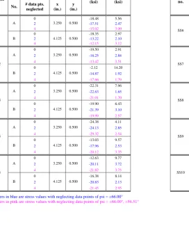
Table 4: Summary of XRD stress results for unblasted samples... 56
viii
LIST OF FIGURES
Figure 1: Diffraction of X-rays by planes of atoms A-A’ and B-B’... 5
Figure 2: Relationship of θ and 2θ... 6
Figure 3: The fourteen Bravais lattices... 7
Figure 4: Diffraction planes parallel to the surface and at an angle φψ... 9
Figure 5a, b: State of stress at point P before and after the introduction of a hole ... 17
Figure 6: Strain gage rosette arrangement to determine residual stress... 19
Figure 7a, b, c: Micro-Measurements residual stress strain gage rosettes... 21
Figure 8a, b: Data-reduction coefficients a and b versus Do/D... 22
Figure 9a, b: Data-reduction coefficients a and b as functions of Z/D and Do/D... 24
Figure 10: Schematic representation of aij ... 26
Figure 11: Model RS-200 Milling Guide... 29
Figure 12: ESPI system setup ... 34
Figure 13: Speckle pattern with fringes ... 35
Figure 14: Hytec, Incorporated PRISM ESPI system... 39
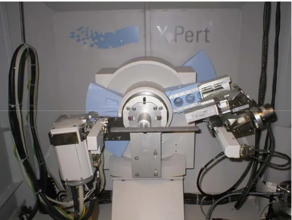
Figure 15: Philips X’Pert PW3040 MPD X-ray diffractometer ... 41
Figure 16: Philips PW3071 sample holder with clip ... 42
Figure 17: Strain-gage hole drilling method setup ... 44
ix
Figure 20: Measurement locations on sample with coordinate system. ... 47
Figure 21: d versus sin2ψ curves of unblasted samples. ... 55
Figure 22: d versus sin2ψ curves of sandblasted samples... 64
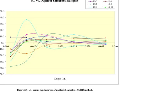
Figure 23: σxx versus depth curves of unblasted samples – SGHD method. ... 68
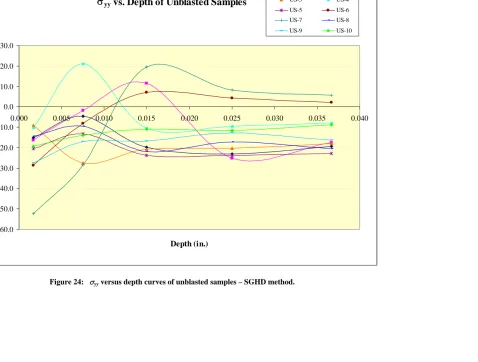
Figure 24: σyy versus depth curves of unblasted samples – SGHD method. ... 69
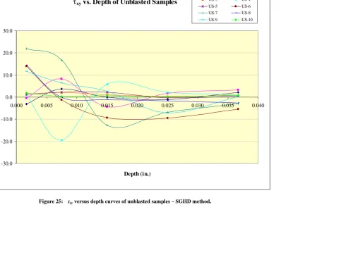
Figure 25: τxy versus depth curves of unblasted samples – SGHD method... 70
Figure 26: σxx versus depth curves of sandblasted samples – SGHD method... 72
Figure 27: σyy versus depth curves of sandblasted samples – SGHD method... 73
Figure 28: τxy versus depth curves of sandblasted samples – SGHD method... 74
Figure 29a, b: Difference in surface conditions on unblasted & sandblasted samples... 77
Figure 30: Fringe patterns acquired from a measurement on unblasted sample... 78
Figure 31: σxx versus depth curves of US-1 to US-5 – ESPI hole drilling method. ... 79
Figure 32: σyy versus depth curves of US-1 to US-5 – ESPI hole drilling method. ... 80
Figure 33: τxy versus depth curves of US-1 to US-5 – ESPI hole drilling method. ... 81
Figure 34: σxx versus depth curves of US-6 to US-10 – ESPI hole drilling method. ... 82
Figure 35: σyy versus depth curves of US-6 to US-10 – ESPI hole drilling method. ... 83
Figure 36: τxy versus depth curves of US-6 to US-10 – ESPI hole drilling method. ... 84
Figure 37: σxx versus depth curves of US-2 – ESPI hole drilling method. ... 85
Figure 38: σyy versus depth curves of US-2 – ESPI hole drilling method. ... 86
Figure 39: τxy versus depth curves of US-2 – ESPI hole drilling method... 87
x
Figure 42: σyy versus depth curves of SS-1 to SS-5 – ESPI hole drilling method... 92
Figure 43: τxy versus depth curves of SS-1 to SS-5 – ESPI hole drilling method. ... 93
Figure 44: σxx versus depth curves of SS-6 to SS-10 – ESPI hole drilling method... 94
Figure 45: σyy versus depth curves of SS-6 to SS-10 – ESPI hole drilling method... 95
Figure 46: τxy versus depth curves of SS-6 to SS-10 – ESPI hole drilling method. ... 96
Figure 47: σxx versus depth curves of SS-2 – ESPI hole drilling method... 97
Figure 48: σyy versus depth curves of SS-2 – ESPI hole drilling method... 98
Figure 49: τxy versus depth curves of SS-2 – ESPI hole drilling method. ... 99
Figure 50: Comparison graphs of US-1. ... 104
Figure 51: Comparison graphs of US-2. ... 106
Figure 52: Comparison graphs of US-3. ... 107
Figure 53: Comparison graphs of US-4. ... 108
Figure 54: Comparison graphs of US-5. ... 109
Figure 55: Comparison graphs of US-6. ... 110
Figure 56: Comparison graphs of US-7. ... 111
Figure 57: Comparison graphs of US-9. ... 112
Figure 58: Comparison graphs of US-10. ... 113
Figure 59: Comparison graphs of SS-1... 116
Figure 60: Comparison graphs of SS-2... 118
Figure 61: Comparison graphs of SS-3... 119
Figure 62: Comparison graphs of SS-4... 120
xi
Figure 65: Comparison graphs of SS-7... 123
Figure 66: Comparison graphs of SS-8... 124
xii
The objectives of this research are to measure residual stress in both unblasted
and sandblasted mild steel specimens by using three different techniques: X-ray
diffraction (XRD), strain-gage hole drilling (SGHD), and electronic speckle pattern
interferometry (ESPI) hole drilling, and to validate the new ESPI hole drilling method by
comparing its measurement results to those produced by the SGHD method.
Both the XRD and SGHD methods were selected because they are accurate and
well-verified approaches for residual stress measurements. The ESPI hole drilling
technique is a new technology developed based on the SGHD technique, without the use
of strain gage. This technique is incorporated into a new product referred to as the
PRISM system, manufactured by Hytec, Incorporated, in Los Alamos, New Mexico.
Each method samples a different volume of material at different depths into the
surface. XRD method is especially different compared to the other two methods, since
XRD only measures stresses at a depth very close to the surface (virtually zero depth).
For this reason, no direct comparisons can be made between XRD and SGHD, as well as
between XRD and ESPI hole drilling. Therefore, direct comparisons can only be made
1. INTRODUCTION
Residual stresses are defined as those stresses that exist in a structural material in
the absence of external forces or thermal gradients. These stresses are introduced into a
component by various manufacturing and fabricating processes (i.e. casting, welding,
machining, molding, heat treatment), as well as in-service repair or modification.
Residual stresses can either have beneficial or detrimental effect on a material,
depending upon their magnitude, sign, and distribution. It is therefore crucial to know
how much locked-in (residual) stresses exist in an object without the presence of any
external loads, especially in the case where fatigue is an important concern. The total
stress that exists within a body is the sum of the residual and applied load stresses [1].
Based on this knowledge, it can be concluded that compressive residual stress increases
the performance capacity of a material, such as fatigue life and crack propagation, while
tensile residual stress promotes fatigue failure.
Residual stress can be measured by several methods, depending on the size and
material of the component to be tested, and the availability, testing speed, and cost of the
equipment. Each method can be categorized as either destructive or non-destructive.
Destructive methods involve the creation of a new state of stress in a material by either
machining or layer removal, detection of the local change in stress by measuring the
strain or displacement, and calculation of residual stress as a function of the measured
deflection, and sectioning. In the case of non-destructive methods, no material
destruction is needed to release the energy or stress stored in it. They mainly involve the
establishment of a relationship between the physical or crystallographic parameters and
the residual stress. The following techniques are considered to be non-destructive: X-ray
diffraction, neutron, ultrasonic, and magnetic methods.
This research compares two commonly used techniques, X-ray diffraction and
strain-gage hole drilling, with one newly-developed electronic speckle pattern
interferometry (ESPI) hole drilling method, to measure the residual stress in both
unblasted and sandblasted mild steel specimens. The X-ray diffraction and strain-gage
hole drilling methods were selected because they are industry standards, representing
non-destructive and destructive techniques, respectively. The equipment used for X-ray
diffraction is very expensive and many are not portable. The size of specimens to be
tested by X-ray diffraction is also limited. When measuring residual stress in large
quantities, the strain-gage hole drilling method is very time consuming and costly. It
requires meticulous work, such as surface preparation, gage installation, and precise hole
drilling. The ESPI hole drilling method can measure residual stress of a material without
any surface preparation. Measurements can be done in a very short amount of time as
well. Residual stress measurement results produced by the strain-gage hole drilling
method are compared to those produced by the ESPI hole drilling to validate this new
technology.
The first three chapters of this paper provide theoretical background and overview
of each method used in this research: X-ray diffraction, strain-gage hole drilling, and
experimental data, which consists of equipment details and settings, as well as test
parameters used in each method. The following chapter contains measurement results
obtained from the three different methods, along with result comparisons. Finally,
2. X-RAY DIFFRACTION METHOD
The X-ray diffraction method enables a nondestructive measurement of residual
stress. It is applicable to crystalline materials with a relatively small (i.e. “fine”) grain
size. This method relies on the elastic deformations within a polycrystalline material to
measure its internal stress.
2.1 BRAGG’S LAW
The fundamental equation of all X-ray diffraction measurements is Bragg’s law,
defined by:
θ λ 2dhklsin
n = (Eq. 2.1)
where n = a whole number of the order of reflection or diffraction
λ = incident radiation wavelength
dhkl = perpendicular distance between adjacent parallel crystallographic planes,
defined by the Miller indices (hkl)
θ = angle of scattering usually referred to as the “Bragg angle”
A crystalline material is made up of many crystals, which are composed of atoms
(d) and the incident radiation wavelength (λ), the planes of atoms can either cause
constructive and/or destructive interference patterns by diffraction [3].
Incident X-ray beams must be parallel, monochromatic, and coherent (in-phase)
in order for diffraction to occur. Figure 1 illustrates the diffraction of X-rays by a crystal
lattice as the basic principle of the Bragg’s law. An “in-phase” X-ray beam of
wavelength λ is incident on the two parallel planes of atoms A-A’ and B-B’ at an angleθ.
Rays 1 and 2 are scattered by atoms P and Q, to yield scattered rays 1’ and 2’ also at an
angleθ to the planes. The difference in path length between the adjacent X-ray beams is
some integral number (n) of radiation wavelength (λ). In other words, SQT =nλ for
constructive interference. Further, by simple geometry,
SQ
nλ= +QT=dhklsinθ +dhklsinθ =2dhklsinθ, which yields the Bragg equation.
Note that the angle θ is the Bragg angle, while the angle 2θ is the diffraction
angle, which is the angle measured experimentally. The relationship between the Bragg
angle (θ) and the experimentally measured diffraction angle (2θ) is shown in Figure 2.
Figure 2: Relationship of θ and 2θ [5].
Destructive interference patterns occur when incident X-ray beams are not
in-phase. In this case, Bragg’s law is not satisfied, and therefore yields a very low-intensity
diffracted beam.
Bragg’s law only defines the diffraction condition for primitive unit cells, which
are those space or Bravais lattices (Figure 3), with lattice points only at unit cell corners,
such as simple cubic and simple tetragonal crystal structures. Nonprimitive unit cells
have atoms at additional lattice sites located along a unit cell edge, within a unit cell face,
or in the interior of the unit cell [5]. As a result, out-of-phase scattering may occur at
certain Bragg angles and some of the diffraction predicted by the Bragg equation does not
Figure 3: The fourteen Bravais lattices [6].
Table 1 lists diffraction rules for the common metal structures. It shows the
Miller indices criteria for several crystal structures in order to produce diffraction, as
Table 1: X-ray diffraction for the common metal structures [5].
Crystal structure Diffraction does not occur when:
Diffraction occurs when:
Body-centered cubic (bcc)
h + k + l = odd number h + k + l = even number
Face-centered cubic (fcc)
h, k, l mixed (i.e., both even and odd numbers)
h, k, l unmixed (i.e., are all even numbers or all odd numbers) Hexagonal close
packed (hcp)
(h + 2k) = 3n, l odd (n is an integer) all other cases
2.2 STRAIN MEASUREMENT AND STRESS DETERMINATION
Each type of strain-free material has a unique inter-planar spacing that yields a
specific diffraction pattern when it is exposed to an X-ray beam. Various manufacturing
and fabricating processes, as well as any external or service loads applied to a body will
cause deformations within the material. These deformations alter the distance between
atomic planes, which in turn cause a shift in the diffraction pattern. The X-ray diffraction
technique measures this shift precisely and gives the change in spacing of the lattice
planes. The strain in the crystal lattice is determined from the change in spacing.
By noting that strain εz and stress σ3 are normal to the specimen surface (the z
direction) and assuming that measurement is conducted within the surface (i.e. σ3 = 0),
the relationship between the inter-planar spacing and strain can be expressed
mathematically as:
0 0
d d dn
z
− =
ε (Eq. 2.2)
If d0 is known, the strain εz can be measured experimentally by determining the high
strain within the surface to be measured by comparing the unstrained inter-planar spacing
(d0) to the strained inter-planar spacing (dn), but is strictly limited to measurements taken
normal to the surface.
Figure 4: Diffraction planes parallel to the surface and at an angle φψ [3].
When a specimen is tilted at a certain angle ψ normal to the surface and/or rotated
at a certain angle φ parallel to the surface in the X-ray diffractometer, the strains along
that direction can be determined by:
0 0
d d
d −
= ψ φψ
ε (Eq. 2.3)
where dψ is the inter-planar spacing of planes at an angle ψ to the surface. Figure 4 is a
schematic showing diffraction planes parallel to the surface and at an angle φψ, where σ1
and σ2 lie in the plane of the specimen surface.
Once strains within the material are known, the stresses associated with them can
(
)
(
1 2)
22 2 2
1cos sin sin
1 υ σ φ σ φ ψ υ σ σ
εφψ = + + − +
E
E (Eq. 2.4)
where E is the Young’s modulus of elasticity and υ is the Poisson’s ratio of the material.
In order to calculate stress in any chosen direction from the inter-planar spacings
determined in a plane normal to the surface and in the direction of the stress to be
measured, strains are considered in terms of inter-planar spacing and they are used to
evaluate the stresses to yield:
(
)
⎟⎟ ⎠ ⎞ ⎜⎜ ⎝ ⎛ − + = n n d d d E ψ φ υ ψ σ 2 sin1 (Eq. 2.5)
σφ is a single stress acting in a chosen direction (i.e. at an angle φ to σ1).
There are several experimental methods to evaluate the stresses within a crystalline
material, including:
a. Two-exposure method
b. Parallel-beam method
c. Sin2ψ method
d. Side-inclination method
e. Variant of the two-exposure method, where the inclined measurement is made at
ψ = 60° rather than at 45° [7].
The Sin2ψ method is the most commonly used. Using this method, measurements are
made at a number of different ψ tilts. At each ψ angle tilt, the inter-planar spacing is
measured. Once measurements are obtained from all ψ tilts, a curve of inter-planar
by obtaining the gradient of the line or elliptical fit, and incorporating the elastic
properties of the material.
Assuming zero stress at d = dn, the stress is given by:
m E
⎟ ⎠ ⎞ ⎜ ⎝ ⎛
+ =
υ σφ
1 (Eq. 2.6)
where m is the gradient of the d versus sin2ψ curve. Equation 2.6 applies only in an ideal
situation, where there is no shear stress present and the stress state within the material is
isotropic. Under these conditions, the curve of d versus sin2ψ is linear.
In the case where shear stresses are present, “ψ splitting” occurs. The curve of d
versus sin2ψ becomes elliptical in shape, with two branches; one corresponds to positive
values of ψ and the other to negative values of ψ. When the stress/strain state within the
material is anisotropic, the curve of d versus sin2ψ becomes oscillatory.
2.3 CHOICE OF X-RAY TUBE ANODE
The choice of an X-ray tube is critical for the measurement of residual stress. In
order to precisely measure the inter-planar spacing (d) within a crystalline material, one
has to select an anode material which gives a suitable Bragg reflection at a sufficiently
high 2θ angle. A radiation is not suitable for a particular kind of crystalline material
when the K-α1 component of the incident beam causes the atoms in the sample to absorb
that energy, and then causes it to produce its own fluorescent X-rays. Fluorescence
causes a very high background and a poor peak-to-background ratio for the resultant data.
If this occurs, it can be improved by using a secondary monochromator or by collecting
All samples tested in this research were mild steel, while the X-ray tube anode
used was copper. A chromium anode would have been a better choice of X-ray tube for
mild steel, but was not available for these measurements. A chromium anode has a
longer wavelength compared to copper. As a result, its radiation does not have sufficient
energy to cause fluorescence. The less energetic chromium anode also penetrates further
into the material compared to the more energetic copper anode. In addition, the planes
used for diffraction are different when a chromium anode is used instead of copper [3].
Regardless of the type of anode chosen, it is critical to measure the stress using a
high 2θ angle – generally greater than 130°. This is because the changes in the d-spacing
due to stress are very small, so the greater the value of θ, the less error in the peak
positioning, as governed by the equation:
θ θcot ∆ − = ∆ d d
(Eq. 2.7)
Table 2 shows recommended test parameters for two common steels, as provided
by Tony Fry of the National Physical Laboratory in Middlesex, UK. Note that the test
parameters are not the same when using different types of anode on the same material.
Table 2: Recommended test parameters for two common steels [8].
Material Radiation Wavelength
(Å) Filter
Peak Plane {hkl}
Peak 2θ Angle (degrees)
Penetration Depth <sin2ψ = 0.3>
(µm)
b.c.c. iron,
ferrite & martensite of iron base materials
Cr-Kα Cu-Kα 2.289649 1.540501 V Monochrom. {211} {222} 156.07 137.13
4.6 - 4.7 1.5 - 1.6
f.c.c. iron,
retained austenite and austenitic base materials
Cr-Kα Cu-Kα 2.289649 1.540501 V Monochrom. {220} {331} 128.84 138.53
2.4 MEASUREMENT PARAMETERS
In order to record diffraction peak in the minimum time possible, generally the
X-ray tube should be operated at its maximum recommended power output. Power settings
should be kept the same for all measurements done for comparison studies. Otherwise,
results will be obtained at different depths below the sample surface. Count time selected
should be long enough to ensure that a well-defined peak is obtained. It is determined
based on the tube and sample characteristics, surface preparation, presence of K-β filter,
as well as the presence of apertures in the incoming or diffracted beam paths. According
to Fitzpatrick et. al [3], doubling the count time improves the counting statistics of each
point in the peak by a factor of 2.
Step size is generally selected in the range of 0.05° to 0.2°. The smaller the step
size, the longer it takes to acquire the peak. However, a smaller step size will give a
more accurate final peak fit. Another measurement parameter to be selected is the
number of tilt angles (ψ). It is recommended to have at least 5 tilts for both positive and
negative ψ angles. If a particular crystalline material does not produce intense peaks,
increasing the number of ψ angle tilts will also improve the accuracy of the final stress
calculation [3].
2.5 POSSIBLE SOURCES OF MEASUREMENT UNCERTAINTY
Several factors that may create uncertainty in a residual stress measurement by
X-ray diffraction method include: elastic constants, instrument alignment, specimen-surface
condition, and operator competence [9]. A study by François, et al. [10] also shows that
the software used to localize the peaks and calculate stress is another variable which can
contribute to the measurement uncertainty of X-ray diffraction.
It is important to distinguish the term “error” from the term “uncertainty”. Error
is the difference between a computed or measured value and a true or theoretically
correct value, while uncertainty is the estimated amount or percentage by which an
observed or calculated value may differ from the true value.
2.6 ADVANTAGES AND DISADVANTAGES OF METHOD
X-ray diffraction is one of the most commonly used methods for residual stress
measurement. It is a nondestructive technique to evaluate surface residual stress.
However, when combined with the layer removal method in order to generate a stress
profile, the method becomes destructive. The measurement time depends on the type of
material of the sample, type of X-ray radiation, and the degree of accuracy required. In
addition to new detector technology, appropriate selection of the X-ray anode and test
settings will greatly reduce the measurement time. Other advantages also include its
versatility, capability to analyze a wide range of materials, and availability of portable
systems.
One of the major disadvantages of this method is that the size and geometry of the
test piece are limited. The sample has to be small enough to fit into the diffractometer
and has to be such that the incident beam can hit the measurement area on the sample,
and still be diffracted to the detector without hitting any obstructions. Rough surface
3. STRAIN-GAGE HOLE DRILLING METHOD
Another popular method to measure residual stress is the strain-gage hole drilling
method. It involves localized removal of stressed material and measurement of strain
relief in the adjacent material using strain gages. The strain-gage hole drilling method is
considered to be a destructive technique because it involves the introduction of a hole
into the test part. In large or thick parts, this method may be considered semi-destructive,
since the small hole introduced into the sample generally will not significantly impair the
structural integrity of the part being tested.
3.1 PRINCIPLES AND THEORY
The introduction of a hole into a component containing residual stresses causes
the surface strains to be relieved locally. The corresponding residual stress within the
material can then be calculated from these relieved strains using formulas derived from
experimental and finite element analyses [7]. There are two different applications of the
strain-gage hole drilling method: through-hole and blind-hole analyses. The theoretical
basis for the hole drilling method applies to the through-hole analysis, which assumes
that a small hole is drilled completely through a thin, wide, flat plate, subjected to
uniform plane stress. However, most practical applications involve the blind-hole
compared to the thickness of the test object. Blind hole analysis is based on the
through-hole analysis [11].
3.1.1 Through-Hole Analysis
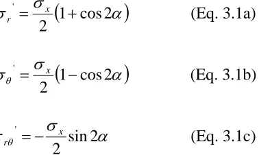
Consider a thin plate with a local area subjected to a uniform residual stress, σx, as
shown by Figure 5a. The state of stress at any point P (expressed in polar coordinates) is:
(
α)
σσ 1 cos2
2
' = x +
r (Eq. 3.1a)
(
α)
σσθ 1 cos2
2 ' − = x (Eq. 3.1b) α σ
τ θ sin2
2
' x
r =− (Eq. 3.1c)
Once a small hole is drilled through it, the state of stress at point P becomes:
α σ
σ
σ 1 3 4 cos2
2 1 1
2 2 4 2
" ⎟ ⎠ ⎞ ⎜ ⎝ ⎛ + − + ⎟ ⎠ ⎞ ⎜ ⎝ ⎛ − = r r r x x
r (Eq. 3.2a)
α σ
σ
σθ 1 3 cos2
2 1 1
2 2 4
" ⎟ ⎠ ⎞ ⎜ ⎝ ⎛ + − ⎟ ⎠ ⎞ ⎜ ⎝ ⎛ + = r r x x
(Eq. 3.2b)
α σ
τ θ 1 3 2 sin2
2 4 2
" ⎟ ⎠ ⎞ ⎜ ⎝ ⎛ − + − = r r x
r (Eq. 3.2c)
where
0
R R
r= and R≥R0. R0 is the hole radius, while R is the arbitrary radius from hole
center [11].
Figure 5a and 5b are illustrations of state of stress at point P before and after the
Figure 5a, b: State of stress at point P before and after the introduction of a hole [11].
The stress relaxation or change in stress at point P due to the hole drilling can be
expressed as:
' "
r r
r σ σ
σ = −
∆ (Eq. 3.3a)
' " θ θ θ σ σ σ = −
∆ (Eq. 3.3b)
' "
θ θ
θ τ τ
τr = r − r
∆ (Eq. 3.3c)
By assuming that the plate is homogeneous and isotropic, and that its stress/strain
behavior is linear-elastic, the above equations can then be substituted into the biaxial
Hooke’s law [11] to yield the following expressions:
(
)
(
)
⎥⎦⎤ ⎢ ⎣ ⎡ + + − + − = α υ α υ σε cos2
1 4 2 cos 3 1 2 1 2 4 2 r r r E x
r (Eq. 3.4a)
(
)
(
)
⎥⎦⎤ ⎢ ⎣ ⎡ + − + − + − = α υ υ α υ σεθ cos2
1 4 2 cos 3 1 2 1 2 4 2 r r r E x
(Eq. 3.4b)
Further, knowing in mind that the relieved radial and tangential strains vary in a
sinusoidal manner at any radius R, Equations 3.4 can be written in a simpler form:
(
α)
σ
εr = x A+Bcos2 (Eq. 3.5a)
(
α)
σ
where the coefficients A, B, and C can be defined as: ⎟ ⎠ ⎞ ⎜ ⎝ ⎛ + −
= 12
2 1
r E
A υ (Eq. 3.6a)
⎥ ⎦ ⎤ ⎢ ⎣ ⎡ − ⎟ ⎠ ⎞ ⎜ ⎝ ⎛ + + −
= 12 34
1 4 2 1 r r E B υ υ (Eq. 3.6b) ⎥ ⎦ ⎤ ⎢ ⎣ ⎡ + ⎟ ⎠ ⎞ ⎜ ⎝ ⎛ + − + −
= 12 34
1 4 2 1 r r E C υ υ υ
(Eq. 3.6c)
The equations above apply to a case of uniaxial residual stress. For biaxial
residual stress, one can perform the above calculations again (but this time in the Y
direction), and then apply the superposition principle. Therefore, when both residual
stresses are present, the relieved radial strain due to plane biaxial residual stress becomes:
(
α)
σ(
α)
(
σ σ) (
σ σ)
α σεr = x A+Bcos2 + y A−Bcos2 = A x + y +B x− y cos2 (Eq. 3.7)
To obtain the principal stresses and the angle α, three independent measurements
of radial strain are acquired. As mentioned earlier, the hole drilling method uses a strain
gage rosette to measure the strain relief caused by the removal of the stressed material
originally in the hole. Figure 6 is an illustration of a strain gage rosette arrangement,
where three radially oriented strain gages are located with their centers at the radius R
Figure 6: Strain gage rosette arrangement to determine residual stress [11].
Based on the gage orientation shown above, the strain for each gage in the rosette
is:
(
σ σ) (
σ σ)
αε1 =A x+ y +B x − y cos2 (Eq. 3.8a)
(
) (
)
cos2(
45o)
2 = σ +σ + σ −σ α +
ε A x y B x y (Eq. 3.8b)
(
) (
)
cos2(
90o)
3 = σ +σ + σ −σ α+
ε A x y B x y (Eq. 3.8c)
The principal stresses and their direction can then be calculated using the following
equations:
(
) (
)
22 1 3 2 1 3 3 1 max 2 4 1
4 ε ε ε ε ε
ε ε
σ = + − − + + −
B
A (Eq. 3.9a)
(
) (
)
22 1 3 2 1 3 3 1 min 2 4 1
4 ε ε ε ε ε
ε ε
σ = + + − + + −
B
A (Eq. 3.9b)
1 3 3 2 1 2 2 tan ε ε ε ε ε α − + −
= (Eq. 3.9c)
Note that the coefficients A and B as defined in Equations 3.6, gives solution of stress
distribution at points with polar coordinates (r,α) around a circular hole through a thin,
give results of the average strain over the grid area. To account for the finite strain gage
area, more accurate A and B coefficients designated by the symbols A and B, can be
obtained by integrating Equations 3.4 over the areas of the respective gage grids.
3.1.2 Blind-Hole Analysis
The blind-hole analysis is an extension of the through-hole analysis. This
application was developed because in practice, test objects are generally not thin, wide,
flat plates subjected to uniform plane stress, as assumed by the through-hole analysis.
The main difference between the two analyses are in the definition of coefficients
A and B. In the blind-hole analysis, each coefficient is a function of E, υ, r, and an
additional coefficient, Z/D. The coefficient Z is the depth of the shallow (blind) hole and
D is the gage circle diameter. According to ASTM E837 [12], which is the standard for
determining residual stress by the strain-gage hole drilling method, the maximum hole
depth is Z/D = 0.4.
Based on the definition of coefficients A and Bdescribed above, it is apparent
that each coefficient is materially and geometrically dependent. Schajer [13] proposed
two new coefficients, a and b, in order to be able to eliminate the material dependency
from A and B coefficients, as defined below:
υ + − =
1 2EA
a (Eq. 3.10a)
B E
Thus, the coefficients A and B can be calculated if the material properties (E and υ) are
known, as well as a and b. The a and b coefficients for many engineering materials
have been determined. Listings for these coefficients are available in Ref. 11, and are
dependent on the strain gage rosette used for the measurement, as well as diameter and
depth of drilled hole.
3.2 COEFFICIENTS FOR MICRO-MEASUREMENTS RESIDUAL STRESS ROSETTES
Vishay Micro-Measurements offers an extensive range of products for precision
measurement of mechanical strains, including bondable strain gages, installation
accessories, and instrumentation. There are three basic strain gage rosette configurations
produced by Micro-Measurements: EA-XX-062RE-120, CEA-XX-062UL-120, and
CEA-XX-062UM-120. Each configuration is shown respectively on Figures 7 below:
Figure 7a, b, c: Micro-Measurements residual stress strain gage rosettes [11].
The RE rosette design is the basic strain gage configuration. The prefix ‘CEA’ of the UL
and UM rosette designs indicates the presence of copper tabs that allow easier soldering
of leads. For the UM rosette design, all grids are located on one side. This geometry
rosette designs have geometrically similar grid configurations, and therefore both designs
have the same material-independent coefficients a and b.
3.2.1 Uniform Residual Stress Calculation
The a and bcoefficients for the RE-, UL-, and UM-type rosettes can be
determined graphically in Figures 8 based on the value of Do/D, where Do is the hole
diameter and D is the is the gage circle diameter. Figure 8a is for types RE- and
UL-rosette, while Figure 8b is for type UM-rosette. In each figure below, the solid lines
apply to full-depth blind holes, while the dashed lines apply to through holes.
Figure 8a, b: Data-reduction coefficients a and b versus Do/D for Measurements Group residual
Note that Figures 8 can only be used when the initial residual stress is uniform with
depth.
3.2.2 Non-Uniform Residual Stress Calculation
In the case where the residual stress varies with depth, the stresses at each partial
depth can be calculated by one of the following methods:
• Integral Method
• Power Series Method
• Incremental Stress Method
• Equivalent Uniform Stress (EUS) Method
The Integral and Equivalent Uniform Stress analysis methods are within the scope of
this study. The Integral method uses finite element calibrations and is recommended for
highly non-uniform stress fields, such as those that exist in sandblasted specimens [14,
15, 16]. It assumes uniform stress within each hole depth increment. The EUS method
uses experimental calibrations, and is an approximate. It produces the same total strain
relief within the total hole depth as the actual non-uniform stress distribution [17].
For the Equivalent Uniform Stress method, the coefficients a and b can be
Figure 9a, b: Data-reduction coefficients a and b as functions of Z/D and Do/D for RE and UL
rosettes [11].
For the Integral method, the total measured strain is the sum of the relieved strains
which originally exist within each of the hole depth increments, as expressed by the
following equation:
∑
= =+
= j i
j j ij
i a P
E p
1
1 υ
, where 1≤ j≤i (Eq. 3.11)
For an isotropic material, p is the “hydrostatic” component of strain measured after “i”
hole depth increments have been drilled, defined by:
(
)
2
1 3 ε ε + =
p for rectangular rosette (Eq. 3.12a)
(
)
3
3 2
1 ε ε
ε + −
=
p for delta strain gage rosette (Eq. 3.12b)
While P is the “hydrostatic” component of stress existing within hole depth increment
(
)
2
x y
P= σ +σ (Eq. 3.13)
The calibration constant aij that relates the stress and strain components can be
determined by:
(
j i) (
j i)
ij a H h a H ha = ˆ , − ˆ −1, (Eq. 3.14)
where hi is the total depth of the hole, and Hj-1 and Hj are the depths at upper and lower
boundaries of that particular hole depth increment. The values of aˆ
(
H,h)
for the RE-,UL-, and UM-type rosettes are tabulated in Ref. 19, page 16. The required (H, h)
combinations can then be determined using bivariate interpolation [19].
For simplification, Equation 3.11 can be expressed in matrix format as:
P a E
p=1+υ (Eq. 3.15)
Similar equations also exist for the other stress and strain components – shear strain 45°
to gage 1 axis (qi), shear strain along gage 1 axis (ti), shear stress to gage 1 axis (Qj), and
shear stress along gage 1 axis (Tj), where
(
)
2 1 3 ε ε − =q for rectangular rosette (Eq. 3.16a)
(
)
3 2 1
3
2 ε ε
ε + −
=
q for delta strain gage rosette (Eq. 3.16b)
(
)
2 2 2
1
3 ε ε
ε + −
=
t for rectangular rosette (Eq. 3.17a)
(
)
3 2 3 ε ε − =(
)
2
x y
Q= σ −σ (Eq. 3.18)
2
xy
T =τ (Eq. 3.19)
Further, q and t can be expressed in matrix formats as follow:
Q b E
q= 1 (Eq. 3.20)
T b E
t= 1 (Eq. 3.21)
Also similar to the calibration constant aij, bij can be determined by:
(
j i) (
j i)
ij b H h b H h
b = ˆ , − ˆ −1, (Eq. 3.22)
The values of bˆ
(
H,h)
for the RE-, UL-, and UM-type rosettes are tabulated in Ref. 19,page 16. The required (H, h) combinations can also be determined using bivariate
interpolation, as described in Ref. 19. To better understand the definition of the
calibration constants, Figure 10 shows a schematic representation of the coefficient aij.
The calibration constant bij have similar definition as the calibration constant aij.
Figure 10: Schematic representation of aij [19].
Once the stresses P, Q, and T, are determined, the state of stress can be calculated
by the following equations:
2 2 min
max,σ =P± Q +T
σ (Eq. 3.23)
2 2 max = Q +T
τ (Eq. 3.24)
⎟⎟ ⎠ ⎞ ⎜⎜ ⎝ ⎛ − − = Q T arctan 2 1
α (Eq. 3.25)
Q P
x = −
σ (Eq. 3.26)
Q P
y = +
σ (Eq. 3.27)
T
xy =
τ (Eq. 3.28)
3.3 INSTRUMENTATION AND SPECIMEN PREPARATION
A portable, battery-powered static strain indicator, supplemented by a precision
switch-and-balance unit allows measurements in the field. The Vishay Measurements
Group Model P-3500 Strain Indicator and SB-10 Switch-and-Balance Unit are ideally
suited for this type of application. One can also use a computerized automatic data
system when measurements are done in the laboratory. Regardless of the type of
instrumentation used, ASTM E837 [12] requires that the instrumentation shall have a
strain resolution of ±2×10⁻⁶, and stability and repeatability of the measurement shall be
at least ±2×10⁻⁶.
Surface preparation is a very critical step in measuring residual stress by the hole
drilling method, particularly incremental hole drilling. The surface of the material to be
mechanical abrasion often generates spurious residual stresses on the surface. In one of
his studies, Prevey [18] confirms that mechanical-abrasive techniques will induce
residual stresses which could alter residual-stress distributions produced by machining,
grinding, or shot-peening. Therefore, the use of abrasive papers should be used only if
absolutely necessary. Electrolytic polishing is the preferred method of surface
preparation. For this method, the prepared area must be flat [19] and a thorough cleaning
and degreasing of the surface is also required.
After the surface preparation, the next step is to install the strain gage rosette. As
with the surface preparation, it is important that the gage installation procedures be of the
highest quality to allow accurate measurement of the small strains. A standard for
surface preparation and rosette installation has been developed and is currently available
in Vishay Measurements Group Instruction Bulletin B-129 [20].
3.4 MEASUREMENT PROCEDURE
Based on Measurements Group Tech Note (TN-503-5) [11], the hole drilling
measurement procedure can be briefly summarized by six basic steps:
a. A three-element strain gage rosette is installed on the test part at the point where
the residual stresses are to be determined. Prior to rosette installation, surface
preparation is conducted at the location where rosette is to be installed.
b. The three gage grids are wired and connected to a static strain indicator, which is
supplemented with a precision switch-and-balance unit.
c. A precision milling guide (Model RS-200, as shown in Figure 11) is attached to
Figure 11: Model RS-200 Milling Guide [21].
d. After zero-balancing the gage circuits, a small and shallow hole is drilled through
the center of the rosette.
e. Relaxed strains readings, which corresponds to the initial residual stress, are
made.
f. Principal residual stresses and their angular orientation are calculated from the
measured strains using the relationships described in Sections 3.1 and 3.2.
3.5 POTENTIAL ERRORS AND UNCERTAINTIES OF METHOD
The potential source of errors and uncertainties of the method [17] are as follows.
• Hole dimensions (diameter, concentricity, profile) – the center of the drilled hole
whichever is greater. More detail on the influence of hole eccentricity can be
found in Ref. 22.
• Hole depth – in material whose thickness is at least 1.2D, the final depth of the
hole should be 0.4D (blind-hole analysis); if material thickness is less than 1.2D, a
hole passing through the entire thickness should be made (through-hole analysis).
• Surface roughness and flatness – should conform to the recommendations
described in Section 3.3.
• Specimen (surface) preparation – should conform to the recommendations
described in Section 3.3.
• Induced stresses from machining the hole – [23]
• Material properties – E and υ
• Incorrect gage selection – gage size (which is closely associated with drill size)
should be considered in relation to the type of stresses present. Small size-gage
should be used on specimen with steep stress gradients, since it gives a more
localized measurement. However, small size-gages are more difficult to handle,
only give limited depth information, and more susceptible to errors associated
with misalignment or surface irregularities.
• Calibration coefficients and method of data analysis used – should conform to the
recommendations described in Sections 3.1 and 3.2.
3.6 ADVANTAGES AND DISADVANTAGES OF METHOD
Strain-gage hole drilling is a simple and widely available method to measure
residual stress in a material. Its instrumentation is portable, and therefore measurements
can be conducted both in the laboratory and in the field. The method is also capable of
testing a wide range of materials, such as metals, polymers, and ceramics. Moreover,
strain-gage hole drilling is a well-established method, experimentally and theoretically.
Specialized precision drilling equipment, along with well-proven experimental
procedures are available for this method. Although a destructive technique, the small
drilled hole on the sample generally will not significantly impair the structural integrity
of the part being tested.
However, the strain-gage hole drilling method can be a tedious and long process.
It requires a significant amount of time to install the rosettes and milling guide. The
surface where the hole is to be drilled has to be prepared according to the standard [20]
available to ensure good bonding between the rosette and the surface. In addition, it is
also important that the hole be drilled exactly in the center of the rosette. These
requirements make residual stress measurement using this technique difficult for field
applications.
Other disadvantages of the method include interpretation of data, and limited
strain sensitivity and resolution. Data interpretation is very important, and often very
difficult. The data analysis method must also be appropriately chosen to match the
expected stress profile of the material being tested.
Several works, including a study done by Gibmeier, et al. [24], confirm that the
in a material, if stress magnitudes are less than 60% of the material yield strength.
Gibmeier, et al. claim that evaluation of residual stresses greater than this limit by the
hole drilling method leads to significant overestimation. In contrast, results from an
experimental study done by Nobre, et al. [25] show that residual stress results obtained
from the strain-gage hole drilling method were still in good agreement with results
obtained from the X-ray diffraction method, even when the magnitudes exceeded the
4. ESPI HOLE DRILLING METHOD
The electronic speckle pattern interferometry (ESPI) hole drilling method was
developed based on the strain-gage hole drilling method. It can measure residual stresses
in a variety of materials, and does not require any surface preparation. Measurements can
also be done in a very small amount of time. Images of the area around the hole are
compared from before and after the hole is drilled. These images, together with
properties of the material being tested and the geometry of the setup, allow determination
of the state of residual stress. Since this method involves the introduction of a hole into
the part being tested, it is considered to be destructive. In large or thick parts, this
method may be considered semi-destructive, since the small hole introduced into the
sample will not significantly impair the structural integrity of the part being tested.
4.1 PRINCIPLES
ESPI hole drilling is a technique capable of providing data on displacements
(shape changes) at the surface of a material by mathematically combining deformation
data, also known as the interferograms, registered digitally before and after the
deformation occurs. In this case, the deformation is caused by drilling a hole in the test
Figure 12 shows the setup of a single beam ESPI system, as illustrated by
Steinzig, et. al [26].
Figure 12: ESPI system setup [26].
The test specimen is exposed to a laser and viewed by a charge-coupled device (CCD)
camera through a lens system and a prism that interferes the object light with a reference
beam from the laser source. The CCD camera records this interference image, which is
then stored in a computer for processing. The interference image illustrates a
random-looking pattern of light and dark speckles, which is caused by the roughness of the
sample and the optics. Images are taken several times before and after a hole is drilled.
Images are stored and processed in the computer to give the corresponding
interferograms on the area around a drilled hole. Figure 13 shows a speckle pattern with
Figure 13: Speckle pattern with fringes.
The mathematical processing of the images is beyond the scope of this paper. More
detailed information can be found in Ref. 26.
4.2 ANALYSIS TECHNIQUE
After deformation data is obtained, the next step is to calculate the associated
residual stress. A number of techniques can be used for this purpose. In 1986, Nelson
and McCrickerd [27] proposed one of the first implementations of combined holographic
interferometry and blind-hole drilling to measure residual stresses in a material. They
derived a method to relate radial displacements measured in three directions of
illumination to the state of residual stress, similar to relations used in the conventional
strain-rosette technique.
Later in 1997, Nelson, et al. [28] further developed this analysis technique, which
was then adapted by Steinzig, et al. [29] in 2001, to be applied to an ESPI system. In this
analysis technique, after the interferograms are acquired, they provide the change in the
illumination beam’s path length (∆P). The value of ∆P corresponds to the surface
displacements as a result of the stress relaxation. The relationship between change in
⎪ ⎪ ⎩ ⎪⎪ ⎨ ⎧ ⎪ ⎭ ⎪ ⎬ ⎫ ⎪ ⎪ ⎩ ⎪⎪ ⎨ ⎧ ⎥ ⎥ ⎥ ⎦ ⎤ ⎢ ⎢ ⎢ ⎣ ⎡ = ⎪ ⎪ ⎭ ⎪⎪ ⎬ ⎫ ∆ ∆ ∆ xy yy xx C C C C C C C C C P P P τ σ σ 33 32 23 22 13 12 31 21 11 3 2 1
(Eq. 4.1)
The Cij values contain constitutive properties, geometric properties, holographic
sensitivity factors, and finite element derived coefficients. ∆Pi is the difference in path
(phase) length between two surface points which are diametrically opposed to one
another, but at the same radial location from the center of the hole, defined by:
(
θ)
−∆(
θ +π)
∆ =
∆Pi P ri, i P ri, i (Eq. 4.2)
Based on the two equations above, it is apparent that three holographic pairs of
data are sufficient to determine the plane state of residual stress at a particular point of
interest (where the hole is drilled).
Since the CCD in an ESPI system typically consists of 256,000 pixel elements,
there are thousands of data points around the hole that are available to determine the state
of stress. Each phase change triad provides an independent stress calculation. The
software processes thousands of these phase change triads, and then averages them to
yield the reported residual stress value.
Another technique used to convert deformation data to calculate residual stress is
the Full Field Least Square (FFLSQ) technique [30]. Unlike previous methods, FFLSQ
is not developed from the through-hole analysis, described in Section 3.1. The
deformation is modeled directly using finite elements, over the full range of each
variable. Interpolation tables can then be generated based on the finite element runs to
provide the best fit to the deformation maps obtained from ESPI. This technique is
4.3 POTENTIAL ERRORS AND UNCERTAINTIES OF METHOD
Since the ESPI hole drilling method is developed based on the strain-gage hole
drilling method, several potential sources of residual stress measurement errors are
identical to those of the strain-gage hole drilling method (Section 3.5). However, some
of the sources of error have been eliminated or reduced. Since there is no strain gage
rosette attached, surface preparation is unnecessary.
In an ESPI system, strains are derived from raw ESPI data on displacement. The
stress is then calculated based on a user-provided modulus of elasticity of the material
being tested. Therefore, any error in the modulus input automatically results into a
relative error in the value of residual stress.
Surface displacements are linearly proportional to the hole depth. Thus, any error
in the hole depth will produce errors in the stresses. Surface displacements are also
linearly dependent on hole diameter. The diameter of the drilled hole depends on the
following factors [31]: drill chuck wobble, machineability of the material, drilling speed
and feed, cutting tool tolerance. Steinzig and Ponchione [32] found that at very low drill
speeds, the resulting holes are not circular; this also contributes to error.
After the hole has been drilled to the test part, the user of an ESPI system defines
the boundaries of the hole using its graphical hole-marking tool to determine the location
of the hole. Numerical experiments were conducted to evaluate the effects of error in
hole center location on the stress results. As described by Ponslet and Steinzig [31],
As in the strain-gage hole drilling method, strains are induced as a hole is drilled
into a part. These induced strains should be kept as low as possible and as limited as
possible in radial extent away from the hole, so that an area can be masked out [31].
Error caused by this factor is difficult to quantify because it varies depending on the
material type and drilling parameters.
Other potential sources of errors are discussed in detail by Ponslet and Steinzig
[31], such as image scale, sensitivity vector, cone beams, wavelength, laser intensity
fluctuations, and drill type of the corresponding ESPI system.
4.4 ADVANTAGES AND DISADVANTAGES OF METHOD
The ESPI hole drilling method eliminates several disadvantages of the strain-gage
hole drilling method (Section 3.6). In addition to its capability to collect data in a short
amount of time in a variety of materials, this method also eliminates the need for strain
gage rosette and the required surface preparation. This method also has the ability to
access smaller regions and information on the displacement field associated with the
introduction of the hole [33].
An ESPI system is fairly portable, and therefore measurements can be easily and
conveniently conducted both in the laboratory and in the field. Figure 14 shows a PRISM
Figure 14: Hytec, Incorporated PRISM ESPI system.
However, since this is a new technology, there are no well-proven experimental
procedures available. More research is required to better establish this method, both
experimentally and theoretically.
Finally, similar to the strain-gage hole drilling method, the small drilled hole on
the sample generally will not significantly impair the structural integrity of the part being
5. EXPERIMENTAL DETAILS
5.1 MATERIAL TESTED
A total of twenty mild steel samples were used in this research. Ten samples were
unblasted and the other ten were sandblasted. All samples have dimensions of 11” x 1” x
¼” (l x w x h), and were cut from the same plate. Therefore all twenty samples have the
same mechanical properties and chemical composition. Table 3 shows the material
details of the samples tested.
Table 3: Mechanical properties and chemical composition of material tested.
Material ASTM A36(01) / A709(01A) / ASME SA36(01ED) / AASHTO M20(01)36
Young’s Modulus (E) 30,733 ksi
Poisson’s ratio (υ) 0.29
Yield Strength (YS) 56,000 – 59,000 psi
Ultimate Tensile Strength (UTS) 69,000 – 73,000 psi
% Elongation 25 – 32
Weight 490 pcf
C Mn P S Si Al Cu Ni Cr Mo Cb V Ti B N Chemical
composition
(% weight) 0.16 0.84 0.010 0.002 0.04 0.025 0.30 0.19 0.14 0.09 0.002 0.005 0.018 0.0001 0.0114
All sandblasted samples were subjected to a white metal blast process using #4 grit silica
5.2 X-RAY DIFFRACTION METHOD
5.2.1 Machine Information and System Settings
All X-ray diffraction measurements were performed using Philips X’Pert
PW3040 MPD (Figure 15), which was set up with a PW3011/20 proportional detector
and PW3071 sample holder with clip (Figure 16).
Figure 16: Philips PW3071 sample holder with clip.
The X-ray source used was a Cu radiation source, with K-α wavelength of
1.5418740 Å. Tube voltage and current were set to 45 kV and 40 mA, respectively.
Apertures used included PW3123/10 monochromator for Cu, divergence and scattering
slits of ½°, receiving slit of 0.30 mm, and soller slit of 0.04 rad.
5.2.2 Test Parameters
Corresponding to the sample stage used, the stress mode was omega stress, with
scan axis of 2θ-omega. Seven tilts for both positive and negative ψ angle were used, as
recommended by Fitzpatrick, et al. [3]. For both types of samples, the diffraction angle
step size was 0.05°, with a counting time of 20 seconds per step. This yielded a scan
speed of 0.0025°/second and a total number of steps of 120. One XRD measurement
For omega stress, the value of maximum ψ angle depended on the start angle of
the scan range (ψ max = [½ * start angle] – 1). Although both unblasted and sandblasted
samples were identical in properties, one yielded a higher angle peak than the other,
which was revealed after running quick scans on both types of the samples. Results show
that high angle peak occurred at 138.5° at {331} plane for the unblasted samples, and
137.0° at {222} plane for the sandblasted samples. Since the high angle peak of each
type of samples was different, the start angle for each type was also different. For
unblasted samples, diffraction angle range was 135.5°-141.5°, which yielded a maximum
ψ angle value of 66.75°. For the sandblasted samples, diffraction angle range was
134°-140° and the maximum ψ angle value was 66°. The difference in the high angle peak for
unblasted and sandblasted samples most likely was caused by the very different surface
conditions. The unblasted samples had smooth surface profiles when compared to the
sandblasted surface, but mill scale was evident at the surface. The sandblasted samples
had no mill scale at the surface, but their surface profile was uniformly uneven.
5.3 STRAIN-GAGE HOLE DRILLING METHOD
5.3.1 Specimen Preparation
Surface preparations and strain gage rosette installations of all twenty samples
were completed according to Vishay Measurements Group Instruction Bulletin B-129
[20]. Strain gage rosettes CEA-06-062UL-120 from Micro-Measurements with grid
centerline diameter of 0.202 in. and a gage length of 0.062 in, were chosen to be used on
![Figure 3: The fourteen Bravais lattices [6].](https://thumb-us.123doks.com/thumbv2/123dok_us/8931932.1846840/20.612.155.494.69.539/figure-fourteen-bravais-lattices.webp)
![Figure 6: Strain gage rosette arrangement to determine residual stress [11].](https://thumb-us.123doks.com/thumbv2/123dok_us/8931932.1846840/32.612.245.404.68.235/figure-strain-gage-rosette-arrangement-determine-residual-stress.webp)
![Figure 11: Model RS-200 Milling Guide [21].](https://thumb-us.123doks.com/thumbv2/123dok_us/8931932.1846840/42.612.231.420.104.319/figure-model-rs-milling-guide.webp)