Development of the probability of return of spontaneous circulation in intervals without chest compressions during out-of-hospital cardiac arrest: an observational study

(1)

Research article

Development of the probability of return of spontaneous

circulation in intervals without chest compressions during

out-of-hospital cardiac arrest: an observational study

Kenneth Gundersen*

1

, Jan Terje Kvaløy

2

, Jo Kramer-Johansen

3

,

Petter Andreas Steen

4,5

and Trygve Eftestøl

1

Address:1_{Department of Electrical and Computing Engineering, University of Stavanger, Stavanger, Norway,}2_{Department of Mathematics and}

Natural Sciences, University of Stavanger, Stavanger, Norway,3_{Institute for Experimental Medical Research, Ulleval University Hospital, Oslo,}

Norway,4_{Faculty Division UUS, University of Oslo, Oslo, Norway and}5_{Division of Prehospital Emergency Medicine, Ulleval University}

Hospital, Oslo, Norway

E-mail: Kenneth Gundersen* - kenneth.gundersen@uis.no; Jan Terje Kvaløy - jan.t.kvaloy@uis.no;

Jo Kramer-Johansen - jo.kramer-johansen@medisin.uio.no; Petter Andreas Steen - p.a.steen@medisin.uio.no; Trygve Eftestøl - trygve.eftestol@uis.no

*Corresponding author

Published: 06 February 2009 Received: 13 January 2009

BMC Medicine2009,7:6 doi: 10.1186/1741-7015-7-6 Accepted: 6 February 2009

This is an Open Access article distributed under the terms of the Creative Commons Attribution License (http://creativecommons.org/licenses/by/2.0), which permits unrestricted use, distribution, and reproduction in any medium, provided the original work is properly cited.

Abstract

Background: One of the factors that limits survival from out-of-hospital cardiac arrest is the interruption of chest compressions. During ventricular fibrillation and tachycardia the electro-cardiogram reflects the probability of return of spontaneous circulation associated with defibrillation. We have used this in the current study to quantify in detail the effects of interrupting chest compressions.

Methods: From an electrocardiogram database we identified all intervals without chest compressions that followed an interval with compressions, and where the patients had ventricular fibrillation or tachycardia. By calculating the mean-slope (a predictor of the return of spontaneous circulation) of the electrocardiogram for each 2-second window, and using a linear mixed-effects statistical model, we quantified the decline of slope with time. Further, a mapping from mean-slope to probability of return of spontaneous circulation was obtained from a second dataset and using this we were able to estimate the expected development of the probability of return of spontaneous circulation for cases at different levels.

Results: From 911 intervals without chest compressions, 5138 analysis windows were identified. The results show that cases with the probability of return of spontaneous circulation values 0.35, 0.1 and 0.05, 3 seconds into an interval in the mean will have probability of return of spontaneous circulation values 0.26 (0.24–0.29), 0.077 (0.070–0.085) and 0.040(0.036–0.045), respectively, 27 seconds into the interval (95% confidence intervals in parenthesis).

Conclusion: During pre-shock pauses in chest compressions mean probability of return of spontaneous circulation decreases in a steady manner for cases at all initial levels. Regardless of initial level there is a relative decrease in the probability of return of spontaneous circulation of about 23% from 3 to 27 seconds into such a pause.

(2)

Background

Recent evidence indicates that cardiopulmonary resusci-tation (CPR) during both in- and out-of-hospital cardiac arrest is characterised by frequent and long interruptions in chest compressions [1, 2]. This reduces vital organ perfusion [3], and in animal experiments, increased length of chest compression pause before shock correlates with reduced rates of return of spontaneous circulation (ROSC) and survival [4-6]. Edelson et al. [7] reported that successful defibrillation, defined as removal of ventricular fibrillation (VF) for at least 5 seconds, was associated with shorter pre-shock pauses in man. Eilevstjønn et al. [8] reported a similar association for shocks with ROSC outcome but only reported the median length of pre-shock pauses for ROSC and no-ROSC pre-shocks. Identifying in detail how pausing in chest compressions affects the vitality of the myocardium, and thereby the probability of ROSC (PROSC) after defibrillation, is important because it

affects treatment priorities before a defibrillation, a vital stage of the resuscitation effort.

During VF and ventricular tachycardia (VT) one can calculate ROSC-predictors from the electrocardiogram (ECG) reflecting thePROSCassociated with defibrillation

[9-12]. In general terms, we can say that ROSC-predictors reflect the coarseness of the ECG or the vitality of the myocardium. ROSC-predictors have been affected posi-tively by compression sequences both in animals [13] and man [14] and negatively by periods with no chest compressions both in animals [15] and man [16]. Unfortunately, we have now realised that the statistical analysis performed in the last article [16] was flawed. This is explained in Appendix 1. In the current work therefore, we reinvestigate the effect of interruptions of chest compressions on PROSC calculated from the ECG. Our

hypothesis was that PROSC decreases during such

inter-ruptions and that the size of this effect may depend on the absolute value of PROSC. We use a ROSC-predictor that

represents the most accurate, currently available estimate ofPROSC[11], and a statistical methodology that properly

handles short time variations of thePROSCestimate and

the fact that thePROSClevel varies from interval to interval

[17]. We handle the problem not solved in Eftestol et al. [16] by applying an adequate regression to the data, representing the underlying trends inPROSCdevelopment,

and use this to derive our results. Further, we compare the results with relevant data from investigations of animal and human sudden cardiac arrest data.

Methods

Data were collected by the respective emergency medical services in an observational prospective study of out-of-hospital cardiac arrest patients in Akershus (Norway), Stockholm (Sweden) and London (UK) in the period

March 2002 to September 2004 [1, 18]. The appropriate ethical boards at each site approved the study, and the need for informed consent from each patient was waived as decided by these boards in accordance with paragraph 26 of the Helsinki declaration for human medical research. The study is registered as a clinical trial at http://www.clinicaltrials.gov/, (NCT00138996). Contin-uous ECG, transthoracic impedance, and chest compres-sion depth measurements were collected using a modified Heartstart 4000 (Phillips Medical Systems, Andover, MA, USA) (Heartstart 4000SP (Laerdal Medi-cal, Stavanger, Norway)) and patient records registered according to the Utstein template [19]. The ECG was obtained through the defibrillator's self-adhesive defi-brillation pads positioned in lead II equivalent positions and the same types of electrodes were used throughout the data collection. The signal was digitally recorded with a sampling rate of 500 samples per second and 16 bits resolution. Before digital sampling the analogue ECG signal was filtered with a second order bandpass filter with passband of 0.9–50 Hz and before analysis a 48 tap lowpass digital filter with an upper passband edge of 30 Hz was applied to the digitised ECG to remove any 50 Hz power line noise. Regarding the mapping-dataset (described below) ROSC was indicated either by a clinically detected pulse or by changes in the transthor-acic impedance >50 mΩcoincident with QRS complexes [1]. Compression depth measurements were used to identify the presence and absence of chest compressions. Further details about registrations and methodology have been given elsewhere [1].

Intervals without chest compressions

We extracted ECG segments from intervals without chest compressions following an interval with compressions. Only segments with VF or VT during both intervals were included. The ECG segments were then divided into 2-second analysis windows centred at 3, 5, 7 and so on up to 27 seconds into the pause, depending on the length of the pause. The first and last 2 seconds of each interval were left out to ensure that the signals were uncorrupted by compression artefacts. We will refer to this dataset as the interval-dataset. ECG segments were manually checked for noise and noisy parts of ECG segments were censored from further analysis. The definition of noise was influence from a pacemaker (regular spikes on the ECG) or short bursts of high frequency signal that visually differ substantially from the surrounding VF or VT. The source of the latter noise form might be electrode noise or muscle artefacts.

Outline of analysis

(3)

the mean-slope (logslope), one of the most accurate indicators ofPROSC[11]. Mean-slope can be viewed as a

measurement of the coarseness of the ECG. High amplitude and frequency of the ECG give high mean-slope values, indicating a high PROSC. If ecg(n) is the

digitised ECG signal, logslopeis defined as

logslope

N ecg n ecg n

N

= ⎛

( )

− −

⎝ ⎜ ⎜

⎞

⎠ ⎟ ⎟

∑

ln 1 ( 1)

1

(1)

Logslopevalues have the desirable property of having an approximate Gaussian distribution, and we thus expected an approximately linear decay with time in untreated VF/VT. A linear mixed-effects model was therefore fitted to logslopeversus time. Then a mapping from logslope to PROSC scale, obtained from a second

clinical dataset (described below), was applied to the f i t t e d l i n e a r m i x e d - e f f e c t s m o d e l f o r e a s i e r interpretation.

Mapping logslope to PROSC

The mapping from logslope to PROSC was found from a

dataset (mapping-dataset) of pre-shock logslope values and corresponding defibrillation outcomes (ROSC or no-ROSC) that has previously been described [20]. The mapping-dataset was collected during cases of out-of-hospital cardiac arrest and ROSC was defined as circulating rhythm for a minimum 10% of the post-shock interval. A marginal logistic regression model for longitudinal data, accounting for correlation between samples from the same patient [21], was fitted to the mapping-dataset using the add-on package 'geepack' to the statistical software R (R Development Core Team, R Foundation for Statistical Computing). The mapping function has the following form:

P logslope e

logslope

e logslope

ROSC

(

)

=

+ ⋅

+ + ⋅

a a

0 1

1 0 1

(2)

a0 and a0 are parameters of the logistic regression estimated during model fitting. The interval-dataset and the mapping-dataset were extracted from the same cardiac arrest episodes. However, since the last 2 seconds of ECG in an interval without chest compressions were not included in the interval-dataset, and we only used the last 2 seconds of ECG before a shock in the mapping-dataset, there is in this respect no overlap of data between the datasets.

Describing logslope development

Using the statistical software S-plus (Insightful Corpora-tion, Seattle, WA, USA), we fitted a linear mixed-effects model to the interval-dataset [17]. The linear mixed-effects model takes into account the fact that the general

level of logslope varies between intervals by allowing individual variation in the regression parameters from interval to interval. The logslopevalues are the response variable in the model, and the development of this described with a polynomial in t, where t is time (seconds) after chest compressions stopped minus 10 seconds (t = torg-10). The subtraction is performed in

order to decorrelate the covariates of the model (t, t2

, etc). Ifiidentifies the interval (cluster), the model for the development oflogslopewith time is given by:

logslopei t k tk U t

k K

ik k

k M

it

( )

= ⋅ + ⋅ +

= =

∑

b

∑

e

0 0

(3)

K is the polynomial degree for the fixed-effects part of the model andMthe degree for the random-effects part (accounting for variations between intervals) andK≥M. Gaussian model residuals εit are assumed and also a

multivariate Gaussian distribution of the random terms Uik,kŒ1, ...,M

f(U_i0,Ui1, ...,UiM) =N(0,Λ) (4)

The S-plus function used to fit the model, lme, has several different possible ways of modelling correlation between residuals within each interval (cluster), and possible heteroschedasticity in the data [17]. We chose the optimal correlation model, variance model (for heteroschedastic data) and the necessary polynomial degree (K and M), in that order, by comparing Akaike information criterion (AIC) values. Polynomial degrees up to four were tested and among possible models with similar AIC values the model of lowest polynomial degrees was chosen. We did not experiment with other variance covariates than the fitted-model value (software default). For mathematical details about the modelling of correlation between residuals and heteroschedastic data we refer to Pinheiro and Bates [17]. After choosing our final model it was validated by plotting normal probability plots for the model residuals and the random terms, the distribution of residuals against time and fitted-model value and the response against fitted values.

Calculating PROSCdevelopment

The linear mixed-effects model was fitted to logslope values due to the statistical properties mentioned above, but we wanted to interpret the implications on thePROSC

scale. More specifically we wanted to find the expected development ofPROSCfor intervals with different starting

values. To avoid the random short time variation in logslope(and PROSC) from influencing the development,

(4)

behaviour. The results are derived from the fitted linear mixed-effects model (not from specific regression lines for each interval) and the obtained mapping from logslope to PROSC. Further descriptions of these

proce-dures are given in Appendix 2.

We present the estimated parameters of the chosen linear mixed-effects model and of the logistic regression model for the logslope to PROSC mapping, along with 95%

confidence intervals (CI) or standard deviation (Std) of estimates for all parameters. Further we present estimates of the expected development with time (into the intervals without compressions) of PROSC for intervals

with different starting values. Approximate 95% CIs for the PROSC developments are derived by drawing 1000

simulated parameter values from the model parameters asymptotic distributions, and then recalculating the resulting PROSCvalues for each simulation. The 95% CI

for the estimated expected PROSC developments are

defined as the 95% CI of PROSCat a given time into an

interval, given a chosenPROSCvalue at the first point of

analysis (3 seconds into the intervals).

Results

Data from 530 defibrillation attempts given to 86 patients were included in the mapping-dataset and used to estimate the logslope to PROSC mapping. In the

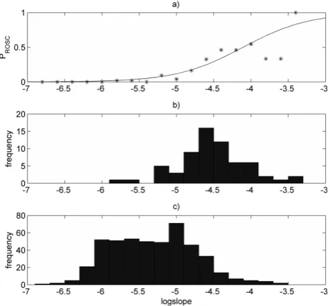
mapping-dataset logslope has an area under the ROSC curve of 0.876 when used to predict which defibrilla-tions will result in ROSC. A histogram of these data is plotted along with the estimated mapping in Figure 1.

Logslope values from 911 intervals without chest com-pressions were included in the interval-dataset and the median interval without chest compressions had five analysis windows. Out of 6229 analysis windows, 17.6% were excluded because of noise in the ECG, leaving 5138. From the complete records of 363 patients, 134 patients had intervals that were included. By comparing AIC values of different candidate models we identified a linear mixed-effects model with an exponential spatial correlation model with nugget effect, polynomial degrees K = 1 and M = 1, and an exponential variance function. Given that a linear model int(polynomials of degree one) was chosen shifting of the time covariate is not necessary, but in order to simplify calculations a time shift of -3 seconds (t = torg-3) was used when

estimating the final model.

Estimated model parameters of the logistic regression model for the logslope to PROSC mapping and of the

chosen linear mixed-effects model are given in Table 1. The logslope value on average decreases 0.00601 per second in our data range (3 to 27 seconds into an

Figure 1

Logslope to PROSCmapping. (a)Mapping (solid line)

estimated with logistic regression model. Point-by-point mapping (asterixes) obtained with a standard histogram technique (based on histograms in (b) and (c)). (b) Histogram of pre-shocklogslopevalues of defibrillations resulting in return of spontaneous circulation (from mapping-dataset). (c) Histogram of pre-shocklogslopevalues of defibrillations resulting in no return of spontaneous circulation (from mapping-dataset).

Table 1: Estimated parameter values of statistical models

Chosen linear mixed-effects model

Parameter Estimate 95% confidence interval

b0 -5.224 [-5.263–5.184]

b1 -0.00601 [-0.00712–0.00490]

Standard deviation (U0) 0.594 [0.564 0.6324]

Standard deviation (U1) 0.00708 [0.00564 0.00889]

Correlation (U0,U1) -0.201 [-0.366–0.0416]

Range 3.11 [1.64 5.88]

Nugget 0.520 [0.401 0.629]

Power -0.598 [-0.805–0.391]

Logistic regression model

Parameter Estimate Standard deviation

a0 9.28 1.51

a1 2.26 0.315

Estimated model parameters of the chosen linear mixed-effects model and the marginal logistic regression model for thelogslopeto probability of return

of spontaneous circulation (PROSC)mapping.b0andb1are the fixed-effects

parameters. Standard deviation (U0), standard deviation (U1) and correlation

(U0,U0) give the properties of the zero-mean bivariate Gaussian distribution

of the random-effects terms. Range and nugget are parameters in the model for correlation between residuals. Power is the parameter in the variance function.a0is the intercept in the logistic regression models linear function,

anda1represents the change in log-odds ratio (ROSC versus no-ROSC)

(5)

interval without chest compressions). The diagnostic plots confirmed that the linear mixed-effects model is adequate for the data.

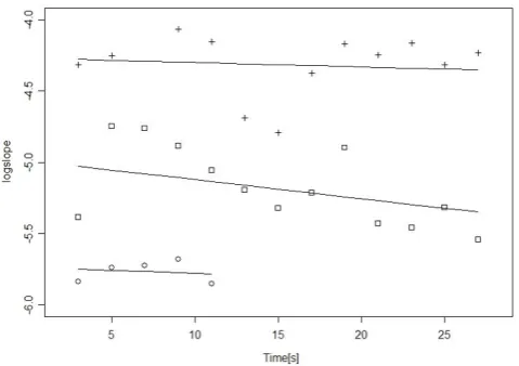
The data in the interval-dataset and how the linear mixed-effects model represents these are illustrated by Figure 2. The figure shows thelogslopevalues and fitted-model values of three intervals. We observe that the intervals are of different length, have logslope values at different levels, and that the fitted lines are allowed to have different intercepts and slopes. The fitted values of Standard deviation(U0), Standard deviation(U1) and

correlation(U0, U1) given in Table 1 describe how the

intercepts and slopes are distributed in our data.

Using Equation (8) in Appendix 2 we computed a set of expected developments of PROSC given different PROSC

values 3 seconds into an interval, shown in Figure 3. According to the b0 parameter, the logslope value 3 seconds into an interval has a Gaussian distribution with mean -5.224 and standard deviation 0.594 (Std(U0)) in

our dataset, and we characterise each development by the quantile the initial logslopevalue (corresponding to the chosen initialPROSCvalue) is at in this distribution.

About 60% of the intervals have initialPROSCbelow 0.1.

Using the approach described in Appendix 2 we estimate that if all the intervals without chest compressions were

shocked with 3 seconds pre-shock pause the meanPROSC

would be 0.126, while with 27 seconds pause it would be 0.0971. The estimated relative decrease in mean PROSC, 1-(0.0971/0.1255)≈0.23, (95% CI: 0.17–0.29) is

comparable with that in each of the developments in Figure 3, meaning that independent of the absolute PROSC level about 23% of the chance of ROSC will be

lost with increasing the pre-shock pause in chest compressions from 3 to 27 seconds.

Discussion

Our analysis shows thatPROSC, as determined from ECG

analysis, decreases in a steady manner with time in VF/ VT intervals without chest compressions for all initial values ofPROSC. This shows that limiting interruption in

chest compressions is important for patients in all states and that every second without perfusion has a negative effect onPROSC. The current results therefore give support

for a strong focus on improving CPR quality.

Unlike the results of Eftestol et al. [16], the current results show thatPROSCdoes not decrease sharply during

the first 5 seconds of an interruption. Therefore, a

Figure 2

Calculated logslopevalues and regression lines from the linear mixed-effects model for three intervals without chest compressions. The linear mixed-effects model is capable of representing that thelogslopevalues (plusses, squares and circles) of different intervals are at different levels (have different intercepts) and decrease or increase at different rates (regression lines have different slopes). The fitted model parameters describe how intercepts and slopes are distributed in the dataset.

Figure 3

Estimated developments of mean probability of return of spontaneous circulation in ventricular fibrillation/ventricular tachycardia intervals without chest compression given different starting values of probability of return of spontaneous circulation. We specified the following starting values (corresponding quantile in our dataset in parenthesis, starting from the top): 0.5(0.97), 0.35(0.92), 0.2(0.80), 0.1(0.6), 0.05(0.38) and 0.01 (0.06). The actual starting value of each development deviates slightly from these values because we must integrate out the residual term in our regression model forlogslope

(6)

pre-shock pause in compressions of a couple of seconds to ensure the safety of EMS personnel, or to perform rhythm analysis on artefact-free ECG, may be acceptable. Concerning safety, pre-shock pauses of 1 to 2 seconds might be sufficient as it has been argued that the risks of accidental defibrillation of resuscitation providers have been over emphasised [22]. Further, the accuracy of rhythm analysis during ongoing compressions might in the future be improved as a result of either improved artefact removal algorithms or of using dedicated ECG recording electrodes generating fewer artefacts than combined recording and defibrillation electrodes [23]. This will also reduce the need for pre-shock pauses in compressions. Although the current results show that pre-shock interruptions in compressions should be minimised, they do not indicate that it is critical, although favourable, for the outcome of resuscitation to compress during defibrillation. This is because there is no indication of a sharp decrease in PROSC during the

first few seconds of an interruption.

The effect of pre-shock interruptions in chest compres-sions on resuscitation outcome or ROSC has also been studied in animals [4-6]. In agreement with the current results all three studies found a clear negative effect of longer pre-shock interruptions. Edelson et al. [7] found strong negative correlation between duration of pre-shock interruptions on first pre-shock success in humans, defined as removal of VF for at least 5 seconds following defibrillation, but no significant effect of pre-shock pause duration on ROSC or survival to hospital discharge. It was stated that one possible reason for this was the limited dataset with lower incidence of ROSC and survival than of shock success with the possibility of a statistical type II error. Eilevstjønn et al. [8] found that the median length of pre-shock interrup-tion of chest compressions for ROSC was 15 seconds versus 18 seconds for no-ROSC shocks (P= 0.008), but did not quantify further the negative effect of increasing length of interruptions.

A limitation of our approach is that the effect was studied indirectly by using the established fact that the PROSCcan be estimated from the ECG waveform [9-12],

instead of by direct analysis of the relation between pre-shock pause length and rate of ROSC. The latter could however, only have identified how the mean probability of ROSC for the population would be influenced by increasing pre-shock pauses in CPR, and could not have identified possible differences in the development for cases with different probabilities of ROSC at the start of the pre-shock interval without chest compressions. Using ECG analysis we can estimate PROSC continuously for

every available interval without chest compressions that follow an interval with chest compressions and,

therefore, estimate the expected development of PROSC

for cases at different starting levels. A further limitation is that we excluded from the analysis all segments where the ECG apparently was affected by a pacemaker and one group of patients was therefore excluded from the analysis. Performing a re-analysis including also the data with noise did however only produce minor changes in the results. At last, the effects of right ventricular dilation and left ventricular contraction occurring during interruptions in compressions, described by Chamberlain et al. [24], may not be reflected in the ECG waveform. The current results may in this respect possibly underestimate the detrimental effect of interrupting compressions.

Conclusion

We have shown that the probability of ROSC estimated from the ECG decreases in a steady manner with increasing pre-shock pauses in chest compressions. Regardless of initial level, there is a relative decrease in the estimated probability of ROSC of about 23% from 3 to 27 seconds, or, in other words, a 1% relative decrease for every second into such a pause.

Abbreviations

AIC: Akaike information criterion; CI: confidence inter-val; CPR: cardiopulmonary resuscitation; ECG: electro-cardiogram; PROSC:probability of return of spontaneous

circulation; ROSC: return of spontaneous circulation; Std: standard deviation; VF: ventricular fibrillation; VT: ventricular tachycardia

Competing interests

PAS is a member of the board of directors for Laerdal Medical. All other authors declare that they have no competing interests.

Authors' contributions

KG conceived the study, developed and performed the analysis and drafted the manuscript. JTK contributed to the development of the analysis methods. JKJ and PAS contributed to the acquisition and preparation of data. TE contributed to the conception of the study and to the preparation of data. All authors have revised and approved the final manuscript.

Appendix 1

(7)

for those with an initially high PROSC value (the first

PROSC value in the segment >0.4), one with medium

initial values (0.25< first PROSC < 0.40), and one with

low initial values (<0.25). After this the development with time of the median of PROSC in the segments in

these three groups was calculated. However, there are quite large random short time variations, or measure-ment noise, in the PROSCestimate used [25], and these

influence the group to which the segments are assigned in the first place. Therefore, for the group of segments with high initial PROSC value a large proportion of the

segments will have high values only at the start of the segment. The median of each group will approach the median of all the segments for the consecutive measurements. We can demonstrate this by re-analysis of

the original data from Eftestol et al. [16], but assign the segments to three groups according to the PROSCvalues

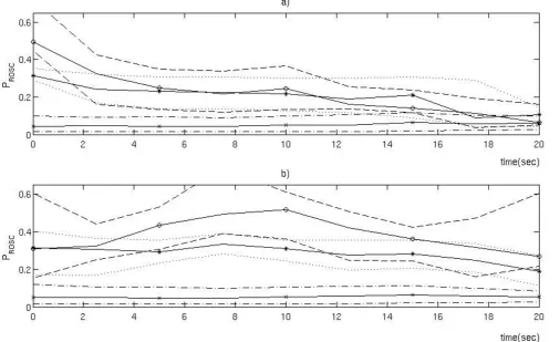
at 10 seconds into the segments rather than according to the initial values. The result of this is shown together with the original plot from Eftestol et al. [16] in Figure 4. If thePROSCestimate from each ECG segment had little

or no random variation between consecutive measure-ments, this modification of the analysis should have little effect on the results. However, changing the time at which the assignment to groups is performed totally changes the plot and we must, therefore, conclude that the analysis is flawed. The inadequate analysis led to unjustified conclusions, most prominently for the 'high' and 'low' subgroups. For cases with a high initial level a dramatic decrease in medianPROSC(from 0.5 to 0.25) with only 5

Figure 4

Two plots illustrating the problem with the analysis performed in the article by Eftestol et al. (a) The original plot from Eftestol et al.'s [16] article where each case was assigned to one of three subgroups ('high', 'medium' and 'low') according to their initial value of probability of return of spontaneous circulation (PROSC). The time axis refers to time into intervals

without compressions. The medianPROSCin each group is represented with a solid line and the various broken lines represent

the 25th and 75th percentiles for each group. The median of the 'high' group differs from the median of the 'medium' group only for the first 5 seconds, and the median of the 'low' group appears to be increasing towards the end. (b) This plot was generated with the same analysis as (a), but here the cases were assigned to the three subgroups according to theirPROSCvalue

at 10 seconds. From the difference between plots (a) and (b), it is evident that the short time random variations in thePROSC

(8)

seconds interruption in chest compressions was falsely indicated, and for the group of cases with low initialPROSC,

representing 85% of the total number of cases, it was indicated that the median PROSC is stable or slightly

increasing during interruptions of up to 20 seconds, despite there being no coronary perfusion. It should be noted that two of the authors (TE and PAS) of the criticised article are also co-authors of the current article.

Appendix 2

If we choose valuexatt= 0 for the regression tologslope, for a hypothetical interval h by choosingUh0 = x -b0, we can

estimate the development of the meanPROSCfor intervals

with a specific starting value. In this way the estimated development is not influenced by the random short time variation inlogslopeatt= 0, represented byεh0. By analogy,

this was the problem with the analysis performed by Eftestol et al. [16]. With the above choice of Uh0 the marginal

distribution of the other random terms is given by:

f U U f x U h UhM

f x _{U h} _{UhM dU}

m h1 hM 0 1

0 1 ,..., , ,..., .. , ,...,

(

)

=

(

−

)

−

(

)

b

b _h_h_1,...._{dU hM} −∞ ∞ ∫ −∞ ∞ ∫ (5) the model for the logslopeattby:

logslopeh t Uh UhM Uh x x k tk U t k

K

hk k k

M

, 1,..., | 0 0

1 1

+ =

( )= + ⋅ + ⋅

= =

∑

b b ++e_ht

(6) and, using Equation (2) for the logslope to PROSC

mapping, the model for PROSCattis given by:

P t U U U x

x k tk k

K

Uhk

ROSC h, , h,..., hM| h

exp

1 0 0

0 1 1 + = ( )= + ⋅ + ⋅ = ∑ + ⋅ b

a a b tt k

k M

ht

x k tk k

K

Uhk tk

= ∑ + ⎛ ⎝ ⎜⎜ ⎞_⎠⎟⎟ ⎛ ⎝ ⎜ ⎜ ⎞ ⎠ ⎟ ⎟ + + ⋅ + ⋅ = ∑ + ⋅ 1

1 0 1

1

e

a a b

exp kk M ht = ∑ + ⎛ ⎝ ⎜⎜ ⎞_⎠⎟⎟ ⎛ ⎝ ⎜ ⎜ ⎞ ⎠ ⎟ ⎟ 1 e (7) Then the expectedPROSCdevelopment given the chosen

initial value can be calculated by:

E P t U x

P t U U U x

ROSC h h

ROSC h h hM h

, , | .. , ,..., | ( ) + = ⎡⎣ ⎤⎦ = + = ( ) 0 0

1 0 0

b

b ⋅⋅ ( )⋅ ( ) −∞

∞

−∞ ∞

∫

fm Uh1,...,UhM f eht dUh1,..,dUhM,deht

(8) By choosing different values for x we can calculate the expected PROSC development for cases with different

starting values. For a given starting value of PROSC, the

corresponding logslope value x is found using Equation (2). If we make no specific choice oflogslopeatt= 0, but modify Equation (8) to integrate out the random intercept Uh0 as well as the other random terms, we

can obtain an estimate for how the meanPROSCdevelops

with time, pooling together cases at allPROSClevels.

Acknowledgements

The efforts of all ambulance personnel and local coordinators of data collection in Akerhus (Hallstein Sørebø), Stockholm (Leiv Svensson) and London (Bob Fellows) are highly appreciated. KG was at the time of the study a PhD student funded by the Norwegian Research Council, project number 27529. TE is the project manager of the same project. The project [1, 18], from which the data originated, was funded by the Norwegian Air Ambulance Foundation (PhD scholarship for JKJ), Regional Health Authorities East (PAS), Laerdal Medical, Stavanger Norway (provided the prototype defibrillators, data collection server, and expenses for extra training related to data collection) and Philips Medical Systems, Andover, MA, USA (original defibrillators). None of these had further involvement in developing the data analysis or writing this article.

References

1. Wik L, Kramer-Johansen J, Myklebust H, Sorebo H, Svensson L, Fellows B and Steen PA:Quality of cardiopulmonary resuscita-tion during out-of-hospital cardiac arrest. JAMA 2005,

293:299–304.

2. Abella BS, Alvarado JP, Myklebust H, Edelson DP, Barry A, O'Hearn N, Hoek Vanden TL and Becker LB: Quality of cardiopulmonary resuscitation during in-hospital cardiac arrest.JAMA2005,293:305–310.

3. Berg RA, Sanders AB, Kern KB, Hilwig RW, Heidenreich JW, Porter ME and Ewy GA: Adverse hemodynamic effects of interrupting chest compressions for rescue breathing during cardiopulmonary resuscitation for ventricular fibrillation cardiac arrest.Circulation2001,104:2465–2470.

4. Sato Y, Weil MH, Sun S, Tang W, Xie J, Noc M and Bisera J:Adverse effects of interrupting precordial compression during car-diopulmonary resuscitation.Crit Care Med1997,25:733–736. 5. Steen S, Liao Q, Pierre L, Paskevicius A and Sjoberg T:The critical

importance of minimal delay between chest compressions and subsequent defibrillation: a haemodynamic explanation. Resuscitation2003,58:249–258.

6. Yu T, Weil MH, Tang W, Sun S, Klouche K, Povoas H and Bisera J:

Adverse outcomes of interrupted precordial compression during automated defibrillation.Circulation2002,106:368–372. 7. Edelson DP, Abella BS, Kramer-Johansen J, Wik L, Myklebust H, Barry AM, Merchant RM, Hoek TLV, Steen PA and Becker LB:

Effects of compression depth and pre-shock pauses predict defibrillation failure during cardiac arrest.Resuscitation2006,

71:137–145.

8. Eilevstjonn J, Kramer-Johansen J and Sunde K:Shock outcome is related to prior rhythm and duration of ventricular fibrilla-tion.Resuscitation2007,75:60–67.

9. Amann A, Rheinberger K and Achleitner U: Algorithms to analyze ventricular fibrillation signals. Curr Opin Crit Care 2001,7:152–156.

10. Eftestol T, Sunde K, Aase SO, Husoy JH and Steen PA:Predicting outcome of defibrillation by spectral characterization and nonparametric classification of ventricular fibrillation in patients with out-of-hospital cardiac arrest. Circulation2000,

102:1523–1529.

11. Neurauter A, Eftestøl T, Kramer-Johansen J, Abella BS, Sunde K, Volker W, Lindner KH, Eilevstjønn J, Myklebust H, Steen PA and Strohmenger H-U:Prediction of countershock success using single features from multiple ventricular fibrillation fre-quency bands and feature combinations using neural net-works.Resuscitation2007,73:253–263.

12. Povoas HP, Weil MH, Tang WC, Bisera J, Klouche K and Barbatsis A:

Predicting the success of defibrillation by electrocardio-graphic analysis.Resuscitation2002,53:77–82.

13. Berg RA, Hilwig RW, Kern KB and Ewy GA: Precountershock cardiopulmonary resuscitation improves ventricular fibrilla-tion median frequency and myocardial readiness for suc-cessful defibrillation from prolonged ventricular fibrillation: A randomized, controlled swine study.Ann Emerg Med2002,

40:563–570.

(9)

defibrillation success during out-of-hospital cardiac arrest. Circulation2004,110:10–15.

15. Brown CG, Dzwoncyzk R and Martin DR:Physiologic measure-ment of the ventricular fibrillation ECG signal: Estimating the duration of ventricular fibrillation.Ann Emerg Med1993,

22:70–74.

16. Eftestol T, Sunde K and Steen PA: Effects of interrupting precordial compressions on the calculated probability of defibrillation success during out-of-hospital cardiac arrest. Circulation2002,105:2270–2273.

17. Pinheiro JC and Bates DM:Mixed-effects Models in S and S-PLUSNew York: Springer; 2000.

18. Kramer-Johansen J, Myklebust H, Wik L, Fellows B, Svensson L, Sorebo H and Steen PA: Quality of out-of-hospital cardiopul-monary resuscitation with real time automated feedback: A prospective interventional study. Resuscitation 2006,

71:283–292.

19. Jacobs I, Nadkarni V, Bahr J, Berg RA, Billi JE, Bossaert L, Cassan P, Coovadia A, D'Este K, Finn J and Halperin H:Cardiac arrest and cardiopulmonary resuscitation outcome reports: update and simplification of the Utstein templates for resuscitation registries: A statement for healthcare professionals from a task force of the international liaison committee on resuscitation (American Heart Association, European Resuscitation Council, Australian Resuscitation Council, New Zealand Resuscitation Council, Heart and Stroke Foundation of Canada, InterAmerican Heart Foundation, Resuscitation Council of Southern Africa).Resuscitation2004,

63:233–249.

20. Gundersen K, Kvaloy JT, Kramer-Johansen J and Eftestol T:

Identifying approaches to improve the accuracy of shock outcome prediction for out-of-hospital cardiac arrest. Resuscitation2008,76:279–284.

21. Diggle P: Analysis of Longitudinal Data Oxford: Oxford University Press; 22002.

22. Perkins GD and Lockey AS: Defibrillation – safety versus efficacy.Resuscitation2008,79:1–3.

23. Fitzgibbon E, Berger R, Tsitlik J and Halperin HR:Determination of the noise source in the electrocardiogram during cardio-pulmonary resuscitation.Crit Care Med2002,30:S148–S153. 24. Chamberlain D, Frenneaux M, Steen S and Smith A:Why do chest

compressions aid delayed defibrillation?. Resuscitation 2008,

77:10–15.

25. Eftestol T, Sunde K, Aase SO, Husoy JH and Steen PA:'Probability of successful defibrillation' as a monitor during CPR in out-of-hospital cardiac arrested patients. Resuscitation 2001,

48:245–254.