INDUCTION MOTOR LOADS
by
Danyal Mohammadi
A thesis
submitted in partial fulfillment
of the requirements for the degree of
Master of Science in Electrical Engineering
Boise State University
DEFENSE COMMITTEE AND FINAL READING APPROVALS
of the thesis submitted by
Danyal Mohammadi
Thesis Title: Dynamic Modeling of Single-Phase Induction Motor Loads
Date of Final Oral Examination: 23 August 2012
The following individuals read and discussed the thesis submitted by student Danyal Mohammadi, and they evaluated his presentation and response to questions during the final oral examination. They found that the student passed the final oral examination.
Said Ahmed-Zaid, Ph.D. Chair, Supervisory Committee
John Chiasson, Ph.D. Member, Supervisory Committee
Jim Browning, Ph.D. Member, Supervisory Committee
I would like to thank my advisor, Professor Said Ahmed-Zaid, for giving me
the opportunity to pursue this research. His guidance and encouragement have been
invaluable. I would also like to thank all the professors at Boise State University who
have taught me so much during my graduate career. In particular, I am grateful for
taking courses from Professor John Chiasson and Professor Jim Browning who were
also members of my supervisory committee.
Finally, I would like to acknowledge the support of the Boise State University
Electrical and Computer Engineering department with a graduate assistantship
dur-ing the 2011-2012 academic year.
Single-phase induction machines are found in various appliances such as
refriger-ators, washing machines, driers, air conditioners, and fans. Large concentrations
of single-phase induction motor loads such as air conditioners and other
motor-compressor loads can adversely impact the dynamic performance of a power system.
An understanding of the dynamics of this type of induction machine is needed to
improve the current state of the art in running power system dynamic studies.
In this thesis, a novel approach of modeling an exact fourth-order model of a
single-phase induction machine is developed that gives credence to the well-known
double revolving-field theory. Using a standard averaging technique, an augmented
seventh-order dynamic model is derived using forward- and backward-rotating
com-ponents. The double-frequency terms causing torque and speed pulsations in the
original model can be recovered as a byproduct of the theory. It is proved that two
three-phase induction machines with their stator windings connected in series but
with opposite phase sequence have the same dynamical behavior as the averaged
single-phase induction machine model. The dynamic and steady-state performances
of the single-phase machine are investigated using the new augmented model and
compared with the exact model.
ABSTRACT . . . vi
LIST OF TABLES . . . x
LIST OF FIGURES . . . xi
LIST OF SYMBOLS . . . xiii
1 Introduction . . . 1
1.1 Research Motivation . . . 1
1.2 Literature Review . . . 3
1.2.1 Double Revolving-Field Theory . . . 3
1.2.2 Dynamic Phasors . . . 6
1.3 Thesis Organization . . . 8
2 Modeling of Single-Phase Induction Machines . . . 10
2.1 Model in Rotor ab-Coordinates . . . 10
2.2 Model in Rotor dq-Coordinates . . . 13
2.3 Augmented Dynamic Model of a Single-Phase Induction Machine . . . 18
2.4 Averaged Dynamic Model of a Single-Phase Induction Machine . . . 20
2.5 Model with Forward- and Backward-Rotating Components . . . 22
2.6 Steady-State Equivalent Circuit . . . 25
3.1 Series-Connected Induction Machines . . . 27
3.1.1 Mathematical Model of Two Series-Connected Three-Phase In-duction Machines in dq-Coordinates . . . 31
3.1.2 State-Space Form of the Voltage Equations of Two Series-Connected Induction Machines . . . 34
3.1.3 Torque Equation . . . 37
3.1.4 Three-Phase Induction Machine Model in a Synchronously-Rotating Reference Frame . . . 39
4 Model Validation and Simulations . . . 42
4.1 Simulation Results . . . 42
4.1.1 Simulation of Exact Fourth-Order dq Model . . . 43
4.1.2 Simulation Comparison of Fourth-Order and Exact Seventh-Order dq Models . . . 44
4.1.3 Simulation Comparison of Fourth-Order and Averaged Seventh-Order dq Models . . . 44
4.1.4 Simulation Comparison of Fourth-Order and Averaged Seventh-Order fb Models . . . 45
4.1.5 Simulation Comparison of Averaged Seventh-Order fb-Model and Seventh-Order Model of Two Three-Phase Series-Connected Induction Machines . . . 46
4.2 Applications . . . 47
4.2.1 Eigenvalue Analysis . . . 47
4.2.2 Participation Factors . . . 49
4.2.4 Recovering Torque and Speed Pulsations from the Averaged
Model . . . 56
4.2.5 Physical Interpretation . . . 60
4.3 Parameters . . . 61
4.4 Experimental Validation . . . 67
5 Conclusion and Recommendations . . . 68
5.1 Conclusion . . . 68
5.2 Recommendations for Future Work . . . 69
A Standard Averaging Theory . . . 73
B Modeling of a Three-Phase Induction Machine . . . 76
B.1 Torque Equation in a Three-Phase Induction Machine . . . 78
4.1 Values of Critical Torque for Each Model . . . 56
4.2 Parameters of Each Single-Phase and Three-Phase Induction Machines 65
1.1 Complex Load Model . . . 1
1.2 Forward and Backward Components of a Stationary Sinusoidal Mag-netic Field . . . 4
1.3 Speed Oscillations . . . 5
1.4 Forward and Backward Torque . . . 6
1.5 Simulation of the Single-Phase Induction Machine Using Dynamic Pha-sors . . . 7
2.1 Stator and Rotor Windings in ab Coordinates . . . 11
2.2 Projecting Rotor Windings to dq Coordinate . . . 13
2.3 Stator and Rotor Windings in dq Coordinate . . . 16
2.4 Equivalent Circuit Representation of a Single-Phase Induction Motor . . 26
3.1 Two Three-Phase Induction Machines Connected in Series . . . 28
4.1 Speed Response of Exact Fourth-Order Model . . . 43
4.2 Speed Responses of Exact Fourth-Order and Seventh-Order dq Models . 45
4.3 Speed Responses of Averaged Order fb-Model and
Seventh-Order Model of Two Three-Phase Series-Connected Induction Machines 46
4.4 Speed Responses of Averaged Order fb-Model and
Seventh-Order Model of Two Three-Phase Series-Connected Induction Machines 47
Model . . . 48
4.6 Speed-Eigenvalue Curve for Averaged Seventh-Order fb-Model . . . 49
4.7 Participation Factors of the Seven States in the Real Eigenvalue Mode 50 4.8 Speed Respond of Seventh-Order and First-Order fb-Models . . . 52
4.9 Speed Responses of Seventh-Order and First-Order fb-Models During Start-Up . . . 53
4.10 Speed Responses of Seventh-Order and First-Order fb-Models with Stator and Rotor Electrical Transients Not Excited . . . 54
4.11 Critical Torque Determination Using Several Models . . . 55
4.12 Exact Stator Currents Isx and Isy from the Exact Seventh-Order dq-Model . . . 56
4.13 Exact Stator Currents Isx and Isy from the Exact Seventh-Order dq-Model . . . 57
4.14 Recovering Speed Oscillations . . . 59
4.15 Magnetic Fields of Motor and Generator . . . 60
4.16 Magnetic Fields of the Single-Phase Induction Machine . . . 61
4.17 Three Single-Phase Induction Machines Coupled on the Same Shaft . . . 62
4.18 Three Quasi-Steady-State Circuits of a Single-Phase Induction Machine 63 4.19 (a) Circuit of Three-Phase Induction Machine (b) Circuit of a Two Three-Phase Induction Machines Connected in Series with Opposite Stator Phase Sequences . . . 64
4.20 Two Three-Phase Induction Machine Connected in Series . . . 67
A.1 Solutions of the Original and Averaged Differential Equations . . . 75
Rs Stator Winding Resistance
Rr Rotor Resistance
ωs Electrical Excitation Frequency
ωm Mechanical Shaft Speed
ω Electrical Shaft Speed
X`s Stator Leakage Reactance
X`r Rotor Leakage Reactance
Xms Mutual Reactance
L`s Stator Leakage Inductance
L`r Rotor Leakage Inductance
Lms Stator Magnetizing Inductance
J Moment of Inertia
CHAPTER 1
INTRODUCTION
1.1
Research Motivation
The adequate modeling of all power system configurations and components is critical
to the determination of accurate power system stability results [1]. Power system
loads are modeled with both static and dynamic load models. Static load models are
represented by constant power, constant current, and constant impedance models, or
some combination of these three types. Induction motor loads are usually separated
using a first-order speed model for small-type motors and by a third-order model for
large-type induction motors.
Modeling the diverse characteristics of a system load gives a more detailed and
accurate system response to voltage and frequency changes [2]. Load types are
decomposed into groups of similar components, as shown in Figure 1.1, where VHV
and T CL respectively stand for the high-voltage bus and a tap-changing-under-load
transformer, and R+jX represents a subtransmission line.
Electrical motors consume about 70% of the electrical energy produced in the
United States. Mostly static models are used to represent induction machines which
accurately model the real power consumption but ignore the reactive power.
There-fore, dynamic models must be used [3]. With stability and voltage problems on the
rise, it has become necessary to include the dynamic characteristics of single-phase
induction machines in the dynamic simulation of power systems.
Single-phase induction machines are commonly found in many household
appli-ances. Most single-phase induction machines are small and built in the fractional
horse-power range. Since single-phase induction motor loads make up a significant
portion of some power systems, it is important to develop accurate models for use in
stability studies.
The dynamic model of the single-phase induction machine currently used exhibits
small double-frequency pulsations superimposed on a steady-state speed. These
double-frequency oscillations exist at an operating point and make it difficult to assess
its small-signal stability. Therefore, it is important to develop an equivalent model
with no oscillations in steady state.
This thesis proposes a new approach to the modeling of a single-phase
induc-tion machine by combining averaging and double revolving-field theories. Applying
this approach to the well-known model of single-phase induction machine yields a
autonomous system with a static equilibrium point. This new averaged model can
be linearized and its eigenvalues can be used to assess the stability of an operating
point.
1.2
Literature Review
How a single-phase induction motor functions has been a topic of discussion for many
years. Even though these theories describe the motor performance well, no adequate
analysis has shown how the various theories compare on the shortcomings [4].
Several theories such as the cross-field theory, the double revolving-field theory,
and dynamic phasors [5] have been proposed to explain the behavior of single-phase
induction machines. In the following sections, the fundamentals of double
revolving-field theory and dynamic phasors will be reviewed.
1.2.1 Double Revolving-Field Theory
The double-field revolving theory was proposed to explain why there is zero shaft
torque at standstill and yet torque once rotated. This theory is based on resolving an
alternating quantity into two components rotating in opposite directions with each
one of them having half the maximum amplitude of the alternating quantity.
Two conditions will be discussed for a single-phase induction machine using the
double revolving-field theory: when the rotor is standstill and when the rotor is
running. When the rotor is at standstill, the torque developed by the forward- and
backward-rotating components is zero.
When the rotor is spinning, as speed increases, the forward flux increases the
The motor quickly accelerates to a final speed near synchronous speed. In the
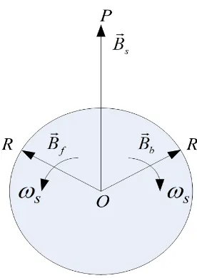
single-phase induction machine shown in Figure 1.2, the stator winding produces
a stationary alternating magnetic field B~s (OP), which can be decomposed into a
forward-rotating field ¯Bf (with magnitude OR) and a backward-rotating field B~b
(with magnitude OR) such that OP=2OR.
Figure 1.2: Forward and Backward Components of a Stationary Sinusoidal Magnetic Field
Based on the double revolving-field theory, the forward and backward components
of the field are rotating in opposite directions and the machine rotates in the forward
direction. Therefore, these components interact with each other at twice the electrical
0.04 0.06 0.08 0.1 0.12 0.14 0.16 0.18 0.2 0.22 358
360 362 364 366 368 370 372 374 376 378
Time (s)
Speed (rad/s)
Original Fourth−Order Model
Figure 1.3: Speed Oscillations
As these two components rotate, they cut the rotor conductors inducing currents
in the short-circuited rotor windings. As shown in Figure 1.4, the torque resulting
from the forward-rotating current components is positive while the torque due to the
backward-rotating components is negative. By symmetry, the net produced torque is
zero at standstill [6] where ω is the machine speed and s is the slip defined as
s = ωs−ω
ωs
−1 −0.8 −0.6 −0.4 −0.2 0 0.2 0.4 0.6 0.8 1 −4
−3 −2 −1 0 1 2 3 4
Slip
Torque (N−m)
Resultant Torque Forward Torque Backward Torque
Figure 1.4: Forward and Backward Torque
1.2.2 Dynamic Phasors
The main idea behind dynamic phasors is to approximate a possibly complex time
domain waveformx(τ) in the intervalτ ∈(t−T, t] with a Fourier series representation of the form
x(τ) =
∞
X
k=−∞
Xk(t)ejkωbτ (1.2)
where
Xk(t) = 1
T
Z t
t−T
x(τ)e−jkωbτdτ = < x >
k (t) (1.3)
and ωb = 2π/T and Xk(t) is the k-th time-varying Fourier coefficient in complex
which provide a good approximation of the original waveform (e.g., k = 0, 1, 2) [5].
In this approach, each of the state variables is expressed in terms of a Fourier series
with time-varying coefficients, and at steady state the dynamic phasors Xk become
constant [7]. This approach can average the state variable oscillations by retaining
some of the harmonics that are often based on physical intuition [5]. Simulating the
single-phase induction machine by this approach yields the green upper envelope and
red lower envelope of the speed response as shown in Figure 1.5.
0 0.1 0.2 0.3 0.4 0.5 0.6 0.7
110 120 130 140 150 160 170 180 190 200
Time (s)
Rotor Speed (rad/s)
Lower Envelope Peak Upper Envelope Peak Averaged Model Exact Model
Figure 1.5: Simulation of the Single-Phase Induction Machine Using Dynamic Phasors
The authors in reference [5] object to the traditional derivation of the equivalent
circuit of a single-phase induction motor that relies upon the principle of superposition
by decomposing a quantity such as magnetic field into the sum of two separate
components. Their argument is justified by the fact that the principle of superposition
In this thesis, we will reconcile the double revolving-field theory and the use of
dynamic phasors by showing that the principle of superposition applies to the torque
equation of an averaged augmented model that will be derived in Chapter 2.
1.3
Thesis Organization
In Chapter 2, we develop a novel approach of modeling a fourth-order model of
a single-phase induction machine based on an exact transformation of the original
electrical variables into well-defined forward and backward components yielding an
augmented seventh-order model that produces an identical dynamic behavior of the
single-phase induction machine under loading transients.
This novel approach is based on standard averaging theory applied to find a
seventh-order averaged model of a single-phase induction machine in which there
are no speed pulsations in steady state.
In Chapter 3, a new model is obtained for two three-phase induction machines
connected in series but with opposite stator phase sequence. The derived
seventh-order model represents both machines coupled on the same shaft and is dynamically
equivalent to the augmented averaged model of a single-phase induction machine with
forward and backward components. These two models clarify the objection in [5] and
yield a seventh-order dynamic model suitable for power system stability studies.
In Chapter 4, several applications are used to validate the developed models. An
eigenvalue analysis is used to confirm the speed or slip at which maximum pull-out
torque occurs. A participation factor analysis shows that the shaft speed is the state
variable associated with a dominant real eigenvalue. This analysis is used to derive
circuit describing the stator and rotor transients. Finally, a transient stability analysis
gives comparable values for the critical torque applied from a no-load condition to
various models of a single-phase induction machine. Chapter 5 summarizes the main
CHAPTER 2
MODELING OF SINGLE-PHASE INDUCTION
MACHINES
In this chapter, the modeling of a single-phase induction machine is developed for the
type commonly referred to as a squirrel-cage motor. In this rotating machine, the
rotor consists of a number of conducting bars short-circuited by conducting rings at
both ends of the squirrel cage.
2.1
Model in Rotor
ab
-Coordinates
A single-phase induction machine has one distributed stator winding and two
equiv-alent rotor windings modeling the squirrel cage. One of the main characteristics
of a single-phase induction machine is that the machine does not produce a torque
at standstill. As with other types of single-phase machines, it needs an auxiliary
winding to produce a non-zero starting torque at standstill that will cause the shaft to
accelerate to near synchronous mechanical speed at no load. A fifth-order differential
vsa = Rsisa+
dλsa
dt (2.1)
0 = Rrira+
dλra
dt (2.2)
0 = Rrirb+
dλrb
dt (2.3)
dθ
dt = ω (2.4)
J p/2
dω
dt = Te−Tm (2.5)
where the label “s” denotes the stator winding, and the labels “ra” and “rb” denote
the rotor phase-aand phase-b windings. The variableλsis the stator flux andλra and
λrb are, respectively, the rotor fluxes of phases a and b. The electrical angle between
the stator winding and the phase-arotor winding is defined asθ. The electromagnetic
torque and the mechanical load torque are defined, respectively, as Te and Tm.
Figure 2.1: Stator and Rotor Windings in ab Coordinates
The auxiliary winding equation is not included in this model because it is
open-circuited by a centrifugal switch when the shaft speed reaches 75 to 80% of its rated
λsa λra λrb =
L`s+Lms Lmscosθ −Lmssinθ
Lmscosθ L`r+Lms 0
−Lmssinθ 0 L`r+Lms isa ira irb (2.6)
whereL`s andL`r are the stator and rotor leakage inductances, respectively, andLms
is the stator magnetizing inductance. It is assumed that the rotor variables have been
referred to the stator side through the use of an effective stator-to-rotor turns ratio.
Assuming an electrically-linear machine, the magnetic co-energy is equal to
Wm0 = 1
2λsaisb+ 1
2λraira+ 1
2λrbirb. (2.7)
Using Equation (2.6), the co-energy is expressed in terms of inductances as
Wm0 = 1
2(L`s+Lms)i 2 sa+
1
2(L`r+Lms) i 2 ra+i
2 rb
+Lmsisa(iracosθ−irbsinθ). (2.8)
The electromagnetic torque developed by the machine is then given by
Te =
∂Wm0 ∂θm
= p
2 ∂W0
m
∂θ (2.9)
whereθm denotes the mechanical angle of rotation related to the electrical angle θby
θ = p
2
θm (2.10)
where p denotes the number of poles per phase. Taking the derivative of Equation
Te =− p
2
Lmsisa(irasinθ+irbcosθ). (2.11)
2.2
Model in Rotor
dq
-Coordinates
The rotor variables of a single-phase induction machine in ab-coordinates are now
transformed to dq coordinates as shown in Figure 2.2, where the fictitious dq windings
appear stationary with respect to the stator.
Figure 2.2: Projecting Rotor Windings to dq Coordinate
The new dq reference frame is stationary with respect to the stator sa-axis. In this
case, the d-axis is aligned with the sa-axis, whereas in another case the q-axis may
be aligned with the sa-axis [8]. To clarify this notation, the model of a single-phase
induction machine will be obtained in both ways. First, the model will be obtained
with the d-axis aligned with the sa-axis. Currents are given by
ird
irq
=
cosθ −sinθ sinθ cosθ
ira
irb
and fluxes by ψrd ψrq =
cosθ −sinθ sinθ cosθ
ψra ψrb
. (2.13)
The inverse transformations are given by
ira irb =
cosθ sinθ
−sinθ cosθ
ird irq (2.14) and ψra ψrb =
cosθ sinθ
−sinθ cosθ
ψrd ψrq
. (2.15)
Using Equations (2.12) through (2.15), a fourth-order model is obtained indq-coordinates
as
vsd = Rsisd+
dλsd
dt (2.16)
0 = Rrird+
dλrd
dt +ωλrq (2.17)
0 = Rrirq+
dλrq
dt −ωλrd (2.18)
dθ
dt = ω (2.19)
J p/2
dω
dt = Te−Tm (2.20)
where vsd = vsa, isd = isa, and λsd = λsa. The new flux-current relationships are
λsd λrd λrq =
L`s+Lms Lms 0
Lms L`r+Lms 0
0 0 L`r+Lms
isd ird irq (2.21)
and the electromagnetic torque simplifies to
Te = −
p
2
Lmsisdirq. (2.22)
This model is expressed using flux linkages and inductances. By using the following
transformation matrix, the model is now expressed in terms of voltage variables and
reactances as ψsd ψrd ψrq
=ωs λsd λrd λrq =
X`s+Xms Xms 0
Xms X`r+Xms 0
0 0 X`r+Xms
isd ird irq (2.23)
where ωs = 120π and 60-Hz reactances have been substituted for inductances. The
final model in dq-coordinates is given by
vsd = Rsisd + 1 ωs
dψsd
dt (2.24)
0 = Rrird+ 1 ωs dψrd dt + ω ωs
ψrq (2.25)
0 = Rrirq+ 1 ωs dψrq dt − ω ωs
ψrd (2.26)
dθ
dt = ω (2.27)
J p/2
dω
dt = Te−Tm (2.28)
ψsd ψrd ψrq =
X`s+Xms Xms 0
Xms X`r+Xms 0
0 0 X`r+Xms
isd ird irq . (2.29)
The electromagnetic torque expression using reactances becomes
Te = −
p
2
Xms
ωs
isdirq. (2.30)
Next, an alternative model found in reference [8] is obtained where the q-axis aligned
with the sa-axis. Consider the q-axis in Figure 2.3, where now it is aligned with
sa-axis.
Figure 2.3: Stator and Rotor Windings in dq Coordinate
The new dq transformations are
irq ird =
cosθ −sinθ
−sinθ −cosθ
and for currents and ψrq ψrd =
cosθ −sinθ
−sinθ −cosθ
ψra ψrb
. (2.32)
for fluxes. Equations (2.31) and (2.32) are the new transformations with the q-axis
aligned with the sa-axis. The final model in these dq coordinates is given by
vsq = Rsisq+ 1 ωs
dψsq
dt (2.33)
0 = Rrird+ 1 ωs dψrd dt + ω ωs
ψrq (2.34)
0 = Rrirq+ 1 ωs dψrq dt − ω ωs
ψrd (2.35)
dθ
dt = ω (2.36)
J p/2
dω
dt = Te−Tm (2.37)
where vsq =vsa, isq =isa, ψsq =ψsa, and
Te = p
2
Xms
ωs
isqird (2.38)
along with the flux-current relationships
ψsq ψrq ψrd =
X`s+Xms Xms 0
Xms X`r+Xms 0
0 0 X`r+Xms
2.3
Augmented Dynamic Model of a Single-Phase Induction
Machine
To develop an augmented model, a stationary dq reference frame is used in this
thesis, where the d-axis is aligned with sa-axis. To lighten up the notation, new
current variables are defined as
is = isd (2.40)
id = ird (2.41)
iq = irq (2.42)
and similarly for flux linkages and voltage variables. The stator winding is excited
with a sinusoidal source voltage of the form
vs(t) =
√
2Vscosωst =
√
2
Vs 2
ejωst+√2
Vs 2
e−jωst. (2.43)
The existence of current solutions is postulated for is(t),id(t), and iq(t) in the form
is(t) =
√
2
Is(t) 2
ejωst+√2
Is∗(t) 2
e−jωst (2.44)
id(t) =
√
2
Id(t) 2
ejωst+√2
Id∗(t) 2
e−jωst (2.45)
iq(t) =
√
2
Iq(t) 2
ejωst+√2
I∗ q(t)
2
e−jωst. (2.46)
where the new complex current solutions are defined in capital letters by Is, Id, and
ψs(t) =
√
2
Ψs(t) 2
ejωst+√2
Ψ∗s(t)
2
e−jωst (2.47)
ψd(t) =
√
2
Ψd(t) 2
ejωst+√2
Ψ∗d(t)
2
e−jωst (2.48)
ψq(t) =
√
2
Ψq(t) 2
ejωst+ √
2 Ψ∗
q(t) 2
e−jωst (2.49)
where Ψs Ψd Ψq =
X`s+Xms Xms 0
Xms X`r+Xms 0
0 0 X`r+Xms
Is Id Iq . (2.50)
Substituting Equations (2.47) through (2.49) into (2.33) yields
√ 2 Vs 2
ejωst + √2
Vs 2
e−jωst=R
s √
2
Is(t) 2 e
jωst
+√2
Is∗(t)
2 e
−jωst
+ 1 ωs d dt √ 2 Ψs(t)
2 e
jωst
+√2
Ψ∗s(t)
2 e
−jωst
. (2.51)
After identifying the coefficients of the linearly-independent functionsejωstande−jωst,
the above differential equation simplify to
Vs = RsIs+
1 ωs
dΨs
dt +jΨs. (2.52)
Repeating this process for the rotor and the speed equations, we end up with the
Vs = RsIs+ 1 ωs
dΨs
dt +jΨs (2.53)
0 = RrId+ 1 ωs
dΨd
dt +jΨd+
ω ωs
Ψq (2.54)
0 = RrIq+ 1 ωs
dΨq
dt +jΨq−
ω ωs
Ψd (2.55)
J (p/2)
dω
dt = −
1 2 p 2 Xm ωs
[IsIq∗+I
∗
sIq +IsIqej2ωst+Is∗I
∗
qe
−j2ωst]−T
m. (2.56)
2.4
Averaged Dynamic Model of a Single-Phase Induction
Machine
After averaging the right-hand sides of (2.53)-(2.56) with respect to timetas explained
in Appendix A, the following autonomous system is obtained
1 ωs
dΨ¯s
dt = −Rs
¯
Is−jΨ¯s+Vs (2.57)
1 ωs
dΨ¯d
dt = −Rr
¯
Id−jΨ¯d−
ω ωs
¯
Ψq (2.58)
1 ωs
dΨ¯q
dt = −RrI¯q−jΨ¯q+ ω ωs
¯
Ψd (2.59)
J (p/2)
dω
dt = −
1 2 p 2 Xms ωs ¯
IsI¯q∗+ ¯I
∗
sI¯q
−Tm (2.60)
where ¯Ψ and ¯I denote the time averaged quantities of the corresponding flux and
current variables, respectively. The constitutive flux-current relationships remain the
same, i.e., ¯ Ψs ¯ Ψd ¯ Ψq =
X`s+Xms Xms 0
Xms X`r+Xms 0
0 0 X`r+Xms
In order to simulate Equations (2.57) through (2.60), they need to be written in
terms of seven real state variables as (ψsx, ψsy, ψdx, ψdy, ψqx, ψqy, ω). This model will
be referred to as the averaged seventh-order dq-model:
1 ωs
dΨsx
dt = −RsIsx+ Ψsy +Vsx (2.62)
1 ωs
dΨsy
dt = −RsIsy −Ψsx+Vsy (2.63)
1 ωs
dΨdx
dt = −RrIdx+ Ψdy−
ω ωs
Ψqx (2.64)
1 ωs
dΨdy
dt = −RrIdy−Ψdx−
ω ωs
Ψqy (2.65)
1 ωs
dΨqx
dt = −RrIqx+ Ψqx+
ω ωs
Ψdx (2.66)
1 ωs
dΨqy
dt = −RrIqy −Ψqy+
ω ωs
Ψdy (2.67)
J (p/2)
dω
dt = −
p
2
Xm
ωs
(IsxIqx+IsyIqy)−Tm (2.68)
with the following flux-current relationships
Ψsx Ψsy Ψdx Ψdy Ψqx Ψqy =
Xs 0 Xms 0 0 0
0 Xs 0 Xms 0 0
Xms 0 Xr 0 0 0
0 Xms 0 Xr 0 0
0 0 0 0 Xr 0
0 0 0 0 0 Xr
Isx Isy Idx Idy Iqx Iqy (2.69)
2.5
Model with Forward- and Backward-Rotating
Compo-nents
The obtained dq-model is now transformed to new coordinates with forward- and
backward-rotating components. Forward and backward flux variables are defined as
¯ Ψf ¯ Ψb = 1 2 1 j
1 −j
¯ Ψd ¯ Ψq (2.70)
Similarly, forward and backward current variables are defined as
¯ If ¯ Ib = 1 j
1 −j
¯ Id ¯ Iq
. (2.71)
The above transformation matrices have been defined differently for fluxes (or
volt-ages) and currents in order to preserve power invariance in the two models. The
inverse transformations are
¯ Ψd ¯ Ψq = 1 1
−j j
¯ Ψf ¯ Ψb (2.72) and ¯ Id ¯ Iq = 1 2 1 1
−j j
¯ If ¯ Ib
. (2.73)
Using Equations (2.70) through (2.73), a new complex model with forward and
1 ωs
dΨ¯s
dt = Vs−Rs
¯
Is−jΨ¯s (2.74)
1 ωs
dΨ¯f
dt = −
Rr 2
¯ If −j
ωs−ω
ωs
¯
Ψf (2.75)
1 ωs
dΨ¯b
dt = −
Rr 2
¯ Ib−j
ωs+ω
ωs
¯
Ψb (2.76)
J (p/2)
dω
dt = −
p
2
Xms
ωs 1 2
¯ Is
2 −jI¯f +jI¯b ∗
+ ¯ Is∗
2 −jI¯f +jI¯b
−Tm
(2.77)
In order to simulate this model, real and imaginary flux and current components are
defined as
¯
Ψs = Ψsx+jΨsy (2.78)
¯
Ψf = Ψf x+jΨf y (2.79)
¯
Ψb = Ψbx+jΨby (2.80)
and
¯
Is = Isx+jIsy (2.81)
¯
If = If x+jIf y (2.82)
¯
Ib = Ibx+jIby. (2.83)
1 ωs
dΨsx
dt = −RsIsx+Vsx+ Ψsy (2.84)
1 ωs
dΨsy
dt = −RsIsy+Vsy−Ψsx (2.85)
1 ωs
dΨf x
dt = −
Rr 2 If x+
ωs−ω
ωs
Ψf y (2.86)
1 ωs
dΨf y
dt = −
Rr 2 If y−
ωs−ω
ωs
Ψf x (2.87)
1 ωs
dΨbx
dt = −
Rr 2 Ibx+
ωs+ω
ωs
Ψby (2.88)
1 ωs
dΨby
dt = −
Rr 2 Iby−
ωs+ω
ωs
Ψbx (2.89)
J (p/2)
dω
dt = −
p 2 Xms ωs 1 2
[IsxIf y−IsyIf x+IsyIbx−IsxIby]−Tm
(2.90)
along with its flux-current relationships,
Ψsx Ψsy
Ψf x
Ψf y
Ψbx Ψby =
Xs 0 X2ms 0 X2ms 0
0 Xs 0 X2r 0 X2r
Xms
2 0
Xr
2 0 0 0
0 Xms
2 0
Xr
2 0 0
Xms
2 0 0 0
Xr
2 0
0 Xms
2 0 0 0
Xr 2 Isx Isy
If x
If y
Ibx Iby (2.91)
2.6
Steady-State Equivalent Circuit
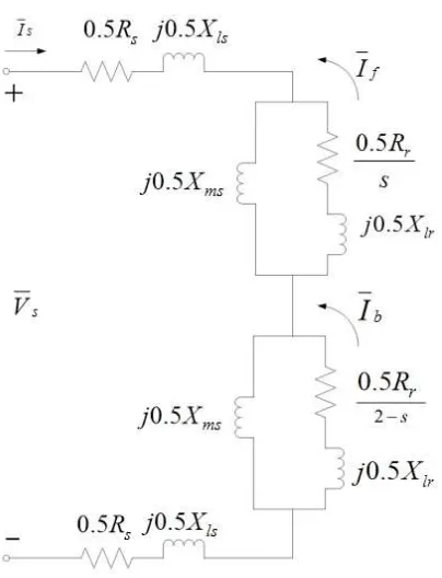
The traditional quasi-steady-state circuit can be derived using several methods in
the literature [6]. The equations of the previous section are now used to derive this
circuit.
This circuit is based on the forward and backward components. The
quasi-steady-state algebraic equations corresponding to Equations (2.74) through (2.76)
are obtained as
0 = Vs−RsI¯s−jΨ¯s (2.92)
0 = −Rr
2 ¯ If −j
ωs−ω
ωs
¯
Ψf (2.93)
0 = −Rr
2 ¯ Ib−j
ωs+ω
ωs
¯
Ψb. (2.94)
Recalling the flux-current relations as
¯
Ψs = (X`s+Xms) ¯Is+j
Xms 2
¯ If +j
Xms 2
¯
Ib (2.95)
¯
Ψf = j
Xms 2 I¯s+j
X`r
2 +
Xms 2
¯
If (2.96)
¯
Ψb = j
Xms 2 I¯s+j
X`r
2 +
Xms 2
¯
Ib (2.97)
and substituting these relations into Equations (2.92)-(2.94) yields the standard
quasi-steady-state of a single-phase induction machine shown in Figure 2.4 and where
s = ωs−ω
ωs
Figure 2.4: Equivalent Circuit Representation of a Single-Phase Induction Motor
The electromagnetic torqueTeis calculated using forward- and backward-rotating
components computed from the equivalent circuit of Figure 2.4 using the following
formulas [6]’:
Tef =
p 2
RrIf2 2sωs
(2.99)
Teb =
p 2
RrIb2 2(2−s)ωs
(2.100)
CHAPTER 3
MODELING OF TWO THREE-PHASE
SERIES-CONNECTED INDUCTION MACHINES
In the previous chapter, the averaged seventh-order model of an induction machine
was derived and expressed in terms of forward and backward components. In this
chapter, it is proved that this model is dynamically equivalent to the model of two
three-phase induction machines connected in series but with opposite stator phase
sequences. The characteristics of this new model will be investigated and compared
to the averaged seventh-order of a single-phase induction machine. For the sake
of consistency, both models will be studied in the synchronously-rotating reference
frame.
3.1
Series-Connected Induction Machines
Figure 3.1 shows two identical three-phase induction machines with their stator
windings connected in series but with opposite stator phase sequences. Each box
Figure 3.1: Two Three-Phase Induction Machines Connected in Series
The rotor windings of each machine are shorted out. From Figure 3.1, it is easily
seen that
isa = isa1 = isa2 (3.1)
isb = isb1 = isc2 (3.2)
isc = isc1 = isb2 (3.3)
where isa, isb, and isc are the source currents. Similarly, isa1, isb1, and isc1 are the
abc stator currents of machine 1, and isa2, isb2, and isc2 are the abc stator currents of
machine 2. In space vector form,
~is = 2
3(isa+ ¯aisb+ ¯a 2i
sc) = ~is1 = ~i∗s2 (3.4)
where ¯a= 16 120o and~i∗
~
vs1 = Rs~is1+ d~λs1
dt (3.5)
0 = Rr~ir1+ d~λr1
dt . (3.6)
From Appendix B,
~λs1 = (L`s+3
2Lms)~is1+ 3 2Lmse
jθ1~i
r1 (3.7)
~
λr1 =
3
2Lms~is1e
−jθ1 + (L
`r+ 3
2Lms)~ir1 (3.8)
Defining~λ0r1 =~λr1ejθ1, we obtain the derivative of ~λ0r1 as
d~λ0r1
dt =
d dt(
~λ
r1ejθ1) = d~λr1
dt e
jθ1 +jω
1~λr1ejθ1 (3.9)
Using Equations (3.6) and (3.9),
d~λ0r1
dt =−Rr~i 0
r1+jω1~λ0r1 (3.10)
where~i0r1 =~ir1ejθ1. To sum up these results, the voltage equations for machine 1 are
given by
~
vs1 = Rs~is1+ d~λ0s1
dt (3.11)
d~λ0r1
dt = −Rr~i
0
r1+jω1~λ0r1 (3.12)
~λ
s1 = (L`s+ 3
2Lms)~is1 + 3 2Lms~i
0
r1 (3.13)
~
λ0r1 = 3
2Lms~is1+ (L`r+ 3 2Lms)~i
0
r1. (3.14)
Similarly, the voltage equations of machine 2 are given by
~
vs2 = Rs~is2+ d~λs2
dt (3.15)
d~λ0r2
dt = −R
0
r~i
0
r2+jω2~λ0r2 (3.16)
along with the new flux-current relationships
~
λs2 = (L`s+
3
2Lms)~is2+ 3 2Lms~i
0
r2 (3.17)
~λ0
r2 = 3
2Lms~is2+ (L`s+ 3 2Lms)~i
0
r2 (3.18)
where~λ0r2 =~λr2ejθ2 and~i0r2 =~ir2ejθ2. With both machines connected in series through
their stator windings, the applied stator voltage~vs can be expressed as
~vs = ~vs1+~vs∗2 = Rs~is1+ d~λs1
dt +Rs~i ∗
s2+ d~λ∗s2
dt . (3.19)
Since~is=~is1 =~i∗s2, we have
~vs = 2Rs~is+
d~λs
dt (3.20)
where the total flux linkages is defined as~λs=~λs1+~λ∗s2. Using Equations (3.13) and
(3.17), this total flux can be expressed in terms of currents as
~λs = ~λs1+~λ∗
s2 = 2(L`s+ 3
2Lms)~is+ 3 2Lms~i
0
r1+ 3 2Lms~i
0∗
The rotor voltage equations remain as they are, that is,
0 = Rr~i0r1+ d~λ0r1
dt −jω1
~λ0
r1 (3.22)
0 = Rr~i0∗r2+ d~λ0∗r2
dt −jω2
~λ0∗
r2 (3.23)
To sum up, the series-connected induction machines are modeled by the following
complex differential voltage equations
~
vs = 2Rs~is+
d~λs
dt (3.24)
0 = Rr~i0r1+ d~λ0r1
dt −jω1
~
λ0r1 (3.25)
0 = Rr~i0∗r2+ d~λ0∗r2
dt −jω2
~
λ0∗r2 (3.26)
together with the flux-current relationships
~λs = 2(L`s+3
2Lms)~is+ 3 2Lms~i
0
r1+ 3 2Lms~i
0∗
r2 (3.27)
~
λ0r1 = 3
2Lms~is+ (L`r+ 3 2Lms)~i
0
r1 (3.28)
~
λ0r2 = 3
2Lms~is+ (L`s+ 3 2Lms)~i
0
r2. (3.29)
3.1.1 Mathematical Model of Two Series-Connected Three-Phase
Induc-tion Machines in dq-Coordinates
The previous model is now transformed intodq-coordinates by decomposing all fluxes
~
λs = λsd+jλsq (3.30)
~λr1 = λrd1+jλrq1 (3.31)
~λr2 = λrd2+jλrq2 (3.32)
for fluxes and
~is = isd +jisq (3.33)
~ir1 = ird1+jirq1 (3.34)
~ir2 = ird2+jirq2. (3.35)
for currents, and substituting Equations (3.30) to (3.35) into Equation (3.27), yields
~λs =λsd+jλsq = 2(L`s+3
2Lms)(isd+jisq) + 3
2Lms(ird1+jirq1) +3
2Lms(ird2−jirq2). (3.36)
Collecting real and imaginary components on both sides of this equation, we obtain
λsd = 2(L`s+
3
2Lms)isd + 3
2Lmsird1+ 3
2Lmsird2 (3.37)
λsq = 2(L`s+
3
2Lms)isq+ 3
2Lmsirq1− 3
2Lmsirq2. (3.38)
A similar decomposition of the rotor flux~λ0r1 of machine 1 yields
~λ0
r1 = λrd1+jλrq1 = 3
2Lms(isd+jisq) + (L`r+ 3
2Lms)(ird1+jirq1)
and
λrd1 = 3
2Lmsisd+ (L`r+ 3
2Lms)ird1 (3.40)
λrq1 = 3
2Lmsisq+ (L`r+ 3
2Lms)irq1. (3.41)
Applying the same procedure for the rotor flux~λ0r2 of machine 2 yields
~λ0
r2 = (λrd2+jλrq2) = 3
2Lms(isd−jisq) + (L`r+ 3
2Lms)(ird2+jirq2) (3.42)
and
λrd2 = 3
2Lmsisd+ (L`r+ 3
2Lms)ird2 (3.43)
λrq2 = −
3
2Lmsisq+ (L`r+ 3
2Lms)irq2. (3.44)
After decomposing all space vector fluxes into real and imaginary components, the
flux-current relationships for the d-axis are given by
λsd
λrd1
λrd2 =
2(L`s+32Lms) 32Lms 32Lms
3
2Lms (L`r+
3
2Lms) 0
3
2Lms 0 (L`r+
3 2Lms)
isd
ird1
ird2 (3.45) and λsq
λrq1
λrq2 =
2(L`s+32Lms) 32Lms −32Lms 3
2Lms (L`r+
3
2Lms) 0
−3
2Lms 0 (L`r+
3 2Lms)
isq
irq1
for the q-axis. Lumping Equations (3.45) and (3.46) together, we obtain the following
composite flux-current relationships
λsd λsq
λrd1
λrq1
λrd2
λrq2 =
2Ls 0 32Lms 0 32Lms 0
0 2Ls 0 32Lms 0 −32Lms
3
2Lms 0 Lr 0 0 0
0 32Lms 0 Lr 0 0
3
2Lms 0 0 0 Lr 0
0 −3
2Lms 0 0 0 Lr
isd isq
ird1
irq1
ird2
irq2 (3.47)
where Ls= (L`s+ 32Lms) and Lr= (L`r+32Lms).
3.1.2 State-Space Form of the Voltage Equations of Two Series-Connected
Induction Machines
State-space variables are defined by decomposing each space vector in the previous
model into real and imaginary parts. By decomposing ~λs, ~λr1, and ~λr2, our model
will have six flux states. First, Equation (3.24),
~
vs = 2Rs~is+
d~λs
dt (3.48)
is replaced with
(vsd+jvsq) = 2Rs(isd+jisq) +
d
dt(λsd+jλsq) (3.49)
dλsd
dt = −2Rsisd+vsd (3.50)
dλsq
dt = −2Rsisq+vsq. (3.51)
Similarly, the rotor flux vector equation for machine 1,
d~λ0r1
dt = −Rr~i
0
r1+jω1~λ0r1 (3.52)
is replaced with
d
dt(λrd1+jλrq1) = −Rr(id1+jiq1) +jω1(λrd1+jλrq1) (3.53)
yielding the following two real rotor differential equations for machine 1
dλrd1
dt = −Rrird1−ω1λrq1 (3.54)
dλrq1
dt = −Rrirq1 +ω1λrd1. (3.55)
For the second machine, its rotor flux vector equation,
d~λ0r2
dt = −Rr~i
0
r2+jω2~λ0r2 (3.56)
is replaced with
d
dt(λrd2+jλrq2) = −Rr(ird2+jirq2) +jω2(λrd2+jλrq2) (3.57)
dλrd2
dt =−Rrird2−ω2λrq2 (3.58)
dλrq2
dt =−Rrirq2+ω2λrd2 (3.59)
To summarize, the following six voltage equations have been obtained
dλsd
dt = −2Rsisd+vd (3.60)
dλsq
dt = −2Rsisq+vq (3.61)
dλrd1
dt = −Rrird1−ω1λrq1 (3.62)
dλrq1
dt = −Rrirq1+ω1λrd1 (3.63)
dλrd2
dt = −Rrird2−ω2λrq2 (3.64)
dλrq2
dt = −Rrirq2+ω2λrd2 (3.65)
Replacing flux variables in Equations (3.60) to (3.65) by voltage variables and
induc-tances by 60-Hz reacinduc-tances yields the following equations
1 ωs
dΨsd
dt = −2Rsisd+vsd (3.66)
1 ωs
dΨsq
dt = −2Rsisq+vsq (3.67)
1 ωs
dΨrd1
dt = −Rrird1−
ω1 ωs
Ψrq1 (3.68)
1 ωs
dΨrq1
dt = −Rrirq1+
ω1 ωs
Ψrd1 (3.69)
1 ωs
dΨrd2
dt = −Rrird2−
ω2 ωs
Ψrq2 (3.70)
1 ωs
dΨrq2
dt = −Rrirq2+
ω2 ωs
Ψrd2 (3.71)
ω = ω1 = ω2. (3.72)
By substituting this speed relation into Equations (3.66) through (3.71), the following
dynamic equations are obtained
1 ωs
dΨsd
dt = −2Rsisd+vsd (3.73)
1 ωs
dΨsq
dt = −2Rsisq+vsq (3.74)
1 ωs
dΨrd1
dt = −Rrird1−
ω ωs
Ψrq1 (3.75)
1 ωs
dΨrq1
dt = −Rrirq1 +
ω ωs
Ψrd1 (3.76)
1 ωs
dΨrd2
dt = −Rrird2−
ω ωs
Ψrq2 (3.77)
1 ωs
dΨrq2
dt = −Rrirq2 +
ω ωs
Ψrd2. (3.78)
3.1.3 Torque Equation
According to Appendix A, the developed electromagnetic torque in a three-phase
induction machine is given by
Te =
3 4
p
2
<e
j3
2Lms~ire jθ~i∗
s+j 3 2Lmse
−jθ~i s~i∗r
(3.79)
which simplifies to
Te =
3 2M
0
sr
p
2
3
2
=m{~is~i∗0r} (3.80)
~i0
r = ~irejθ (3.81)
is a space vector in the stationary stator reference frame. Recalling Equations (3.33)
to (3.35) and decomposing them using real and imaginary components, we get
~is1 = isd1+jisq1 = ~is = isd+jisq (3.82)
~i∗
s2 = isd2−jisq2 = ~is = isd+jisq. (3.83)
Substituting these current components into the torque expression for the first machine
yields
Te1 =
p
2
3
2Lms 3 2
=m{~is1~i0∗r1} (3.84)
=
3 2Lms
p 2 3 2
=m{(isd1+jisq1)(i0rd1−ji
0
rq1)} (3.85)
=
3 2Lms
p 2 3 2
=m{(isd+jisq)(i0rd1−ji
0
rq1)} (3.86)
=
3 2Lms
p 2 3 2
(isqi0rd1−isdi0rq1) (3.87)
Similarly, the torque produced by the second machine is given by
Te2 =
p
2
3
2Lms 3 2
=m{~is2~i0∗r2} (3.88)
= p
2
3
2Lms 3 2
=m{(isd2+jisq2)(i0rd2−ji
0
rq2)} (3.89)
= p
2
3
2Lms 3 2
=m{(isd−jisq)(i0rd2−ji
0
rq2)} (3.90)
= −
3 2Lms
p 2 3 2
Since the two machines are rigidly coupled through the shaft, the aggregate torque
equation is given by
J (p/2)
dω
dt =Te1+Te2−Tm (3.92)
whereJ is the sum of the inertias of both machines andTm is the applied mechanical
torque.
Substituting Equations (3.87) and (3.91) into (3.92) yields the following torque
equation
J p/2
dω
dt =
p
2
9Lms 4
(isqi0rd1−isdi0rq1−isqi0rd2−isdi0rq2)−Tm (3.93)
3.1.4 Three-Phase Induction Machine Model in a Synchronously-Rotating
Reference Frame
In this section, the complete model derived in a stationary reference frame is
repro-duced below using voltage variables as
1 ωs
dΨsd
dt = −2Rsisd+vsd (3.94)
1 ωs
dΨsq
dt = −2Rsisq+vsq (3.95)
1 ωs
dΨrd1
dt = −Rrird1−
ω ωs
Ψrq1 (3.96)
1 ωs
dΨrq1
dt = −Rrirq1+
ω ωs
Ψrd1 (3.97)
1 ωs
dΨrd2
dt = −Rrird2−
ω ωs
Ψrq2 (3.98)
1 ωs
dΨrq2
dt = −Rrirq2+
ω ωs
Ψrd2 (3.99)
J (p/2)
dω
dt =
p
2
9Msr 4
[(isqi0rd1−isdi0rq1)−(isqi0rd2+isdi0rq2)]−Tm
.
Since the synchronously-rotating reference frame is a special and useful reference
frame for running simulations, the previous model is now transformed to this reference
frame using a standard procedure as
1 ωs
dΨsd
dt = −2Rsisd+ Ψsq+vsd (3.101)
1 ωs
dΨsq
dt = −2Rsisq−Ψsd+vsq (3.102)
1 ωs
dΨrd1
dt = −Rrird1−
ω ωs
Ψrq1+ Ψrq1 (3.103)
1 ωs
dΨrq1
dt = −Rrirq1+
ω ωs
Ψrd1−Ψrd1 (3.104)
1 ωs
dΨrd2
dt = −Rrird2−
ω ωs
Ψrq2−Ψrq2 (3.105)
1 ωs
dΨrq2
dt = −Rrirq2+
ω ωs
Ψrd2+ Ψrd2 (3.106)
J (p/2)
dω
dt =
p
2
9Xms 4ωs
[(isqi0rd1−isdi0rq1)−(isqi0rd2+isdi0rq2)]−Tm
(3.107)
where the new variables have kept the same names in both reference frames. After
some manipulations, this model simplifies to
1 ωs
dΨsd
dt = −2Rsisd+ Ψsq+vsd (3.108)
1 ωs
dΨsq
dt = −2Rsisq−Ψsd+vsq (3.109)
1 ωs
dΨrd1
dt = −Rrird1+
ωs−ω
ωs
Ψrq1 (3.110)
1 ωs
dΨrq1
dt = −Rrirq1−
ωs−ω
ωs
Ψrd1 (3.111)
1 ωs
dΨrd2
dt = −Rrird2−
ωs+ω
ωs
Ψrq2 (3.112)
1 ωs
dΨrq2
dt = −Rrirq2+
ωs+ω
ωs
J (p/2)
dω
dt =
p
2
9Xms 4ωs
[(isqi0rd1−isdi0rq1)−(isqi0rd2+isdi0rq2)]−Tm.
(3.114)
The flux-current relationships remain as in (4.38), that is
Ψsd Ψsq
Ψrd1
Ψrq1
Ψrd2
Ψrq2 =
2Xs 0 32Xms 0 32Xms 0
0 2Xs 0 32Xms 0 −32Xms
3
2Xms 0 Xr 0 0 0
0 32Xms 0 Xr 0 0
3
2Xms 0 0 0 Xr 0
0 −3
2Xms 0 0 0 Xr
isd isq
ird1
irq1
ird2
irq2 (3.115)
CHAPTER 4
MODEL VALIDATION AND SIMULATIONS
4.1
Simulation Results
In this section, the dynamic performance of the models derived in previous chapters
is compared. The models simulated in this chapter include the following:
• Exact fourth-order dq model;
• Exact seventh-order dq model;
• Averaged seventh-order dq model;
• Averaged seventh-order fb model;
• Seventh-order model of two three-phase induction machines.
The auxiliary winding of a single-phase induction machine has been neglected in
all of these simulations. All models will be simulated with an initial speed condition
of 75% of rated speed and with zero initial currents.
A load torque Tm = 2.5 N-m is applied at t = 0.5 s and removed at t = 1.5 s.
All models are simulated using classical fourth-order Runge-Kutta method with a
4.1.1 Simulation of Exact Fourth-Order dq Model
Figure 4.1 shows the dynamic speed response of a single-phase induction machine
using its original fourth-order model described by Equations (2.33) through (2.35)
and (2.37). The following initial conditions are used in this simulation:
ψs(0)
ψd(0)
ψq(0)
ω(0)
=
0
0
0
0.75ωs
. (4.1)
0 0.2 0.4 0.6 0.8 1 1.2 1.4 1.6 1.8 2
260 280 300 320 340 360 380
Time (s)
Speed (rad/s)
Figure 4.1: Speed Response of Exact Fourth-Order Model
As expected, the steady-state speed pulsates at twice the synchronous frequency
for both no-load and loaded conditions. Based on the characteristics of an induction
a lower value and, after removing the load at t = 1.5 s, the speed of the machine
returns to its no-load steady-state value.
4.1.2 Simulation Comparison of Fourth-Order and Exact Seventh-Order
dq Models
To simulate the seventh-order dq-model, the initial conditions used are
ψsx(0)
ψsy(0)
ψdx(0)
ψdy(0)
ψqx(0)
ψqy(0)
ω(0) = 0 0 0 0 0 0
0.75ωs . (4.2)
Figure 4.2 illustrates the speed responses of both the fourth-order and
seventh-order models in dq-coordinates. This figure shows that both models yield identical
dynamic speed responses verifying the validity of the augmented model.
4.1.3 Simulation Comparison of Fourth-Order and Averaged
Seventh-Order dq Models
Equations (2.57) through (2.60) describe the averaged seventh-order model of a
single-phase induction machine in dq coordinates. By averaging the double-frequency terms
( ej2ωst and e−j2ωst ) in the exact seventh-order model, a model where the speed is
0 0.2 0.4 0.6 0.8 1 1.2 1.4 1.6 1.8 2 260
280 300 320 340 360 380
Time (s)
Speed (rad/s)
Original Fourth−Order Model
Seventh−Order Model in dq coordinates
Figure 4.2: Speed Responses of Exact Fourth-Order and Seventh-Order dq Models
Transforming the dq-model to a model with forward and backward components
using the defined power-invariant transformation matrices in (2.70) and (2.73) does
not change the dynamic speed response that is shown in Figure 4.2.
4.1.4 Simulation Comparison of Fourth-Order and Averaged
Seventh-Order fb Models
In this section, we compare the speed responses of the original fourth-order model
and the averaged seventh-order fb-model. As expected, the speed of the machine is
constant during steady state and without oscillations as shown in Figure 4.3 in the
averaged model.
During the initial electrical transient, the speed of the averaged model does not
0 0.2 0.4 0.6 0.8 1 1.2 1.4 1.6 1.8 2 240
260 280 300 320 340 360 380
Time (s)
Speed (rad/s)
Original Fourth−Order Model Averaged Seventh−Order fb−Model
Figure 4.3: Speed Responses of Averaged Seventh-Order fb-Model and Seventh-Order Model of Two Three-Phase Series-Connected Induction Machines
and rotor electrical transients are differently excited in both models. Following the
mechanical disturbance at t = 0 s, the stator and rotor electrical transients are not
excited and in this model the averaged speed follows the average of the exact pulsating
speed.
4.1.5 Simulation Comparison of Averaged Seventh-Order fb-Model and
Seventh-Order Model of Two Three-Phase Series-Connected
Induc-tion Machines
The simulations of the fb-model of a single-phase induction machine and two
three-phase series-connected induction machines yield interesting results. Figure 4.4 clearly
shows that both models are superimposed with identical dynamic speed responses
0 0.2 0.4 0.6 0.8 1 1.2 1.4 1.6 1.8 2 240
260 280 300 320 340 360 380
Time (s)
Speed (rad/s)
Averaged Seventh−Order fb−Model
Model of Two Three−Phase Induction Machines
Figure 4.4: Speed Responses of Averaged Seventh-Order fb-Model and Seventh-Order Model of Two Three-Phase Series-Connected Induction Machines
4.2
Applications
In this section, the small-signal stability of the averaged seventh-order fb-model using
eigenvalue analysis is studied. At a certain operating speed, the system will become
unstable. As will be shown, this instability occurs when one real eigenvalue becomes
zero at the maximum pull-out torque.
4.2.1 Eigenvalue Analysis
For a system with n state variables, the eigenvalues of an n×n matrix A are the n solutions of the characteristic equation
Using the machine parameters in Table 4.2, Equations (2.84) to (2.90) yields a 7×7 system matrix A for the averaged seventh-order fb-model. The maximum torque of
0 50 100 150 200 250 300 350 400
0 0.5 1 1.5 2 2.5 3
X: 275 Y: 2.615
Speed (rad/s)
Torque (N−m)
Torque−Speed Characteristic Curve
Figure 4.5: Torque-Speed Characteristic Curve for Averaged Seventh-Order fb-Model
about 2.6 (N-m) occurs at an electrical speed of 275 (rad/s) as shown in Figure 4.5.
The machine cannot handle additional torque and it is expected that the machine will
stall for a torque larger than 2.6 (N-m). This analysis assumes a constant mechanical
load torque.
Figure 4.6 shows the real eigenvalue corresponding to each operating speed. At
the speed of 275 (rad/s), this eigenvalue becomes zero, verifying the instability of the
0 50 100 150 200 250 300 350 400 −120
−100 −80 −60 −40 −20 0 20
X: 275 Y: −0.03666 X: 274
Y: 0.2939
Speed (rad/s)
Eigenvalues
Figure 4.6: Speed-Eigenvalue Curve for Averaged Seventh-Order fb-Model
4.2.2 Participation Factors
In the study of dynamic systems, it may be necessary to construct reduced-order
models for dynamic stability studies by retaining only a few modes of interest. It
then becomes important to determine which state variables significantly participate
in the selected modes.
Verghese et al. [9] proposed a tool known as a participation factor to calculate a
dimensionless measure of how much each state variable contributes to a given mode.
Given a linear system
˙
x = Ax (4.4)
the participation factor is defined as
pki =
wkivki
wt ivi
(4.5)
wherewki andvki are thekth entries in the left and right eigenvectors associated with
witvi = n X
k=1
pki = 1. (4.6)
In order to obtain these participation factors for the sole real mode, the seventh-order
fb-model is linearized for a defined speed range from 0 to ωs. For example, the
participation factors at ω = 350 (rad/s) are
(pk7)T =
−0.224 0.014 −0.263 0.294 −0.007 0.008 0.977
(4.7)
indicating that Ψsy, Ψf y, and ω are the dominant variables in this real mode.
0 50 100 150 200 250 300 350 400 −0.4
−0.2 0 0.2 0.4 0.6 0.8 1
X: 275 Y: 0.9375
Participation Factor
All States in the Seventh Model
Speed (rad/s)
sx sy fx fy bx by w
Figure 4.7: Participation Factors of the Seven States in the Real Eigenvalue Mode
As shown in Figure 4.7, the seventh speed state has a large participation factor
region. It is also interesting that at ω = 275 (rad/s) the machine becomes unstable.
Using a participation factor analysis where p77 has a greater value compared
to the other states, the slowest state corresponding to the dominant eigenvalue is
determined as the speed of the machine. This suggests that the stator and rotor
electrical transients are much faster than the rotor speed. Eliminating these fast
electrical variables by using a quasi-steady circuit model, a first-order speed model
of the machine can be derived. By setting the left-hand sides of the stator and rotor
electrical transients to zero, the averaged fb-model in (2.62) to (2.68) becomes
0 = −RsIsx+ Ψsy+Vsd (4.8)
0 = −RsIsy−Ψsx+Vsq (4.9)
0 = −Rr
2 If x+
ωs−ω
ωs
Ψf y (4.10)
0 = −Rr
2 If y−
ωs−ω
ωs
Ψf x (4.11)
0 = −Rr
2 Ibx+
ωs+ω
ωs
Ψby (4.12)
0 = −Rr
2 Iby−
ωs+ω
ωs
Ψbx (4.13)
J (p/2)
dω
dt = −
p
2
Xms
ωs 1 2
[IsxIf y−IsyIf x+IsyIbx−IsxIby]−Tm.
(4.14)
After solving the above equations, the first-order speed model is
J (p/2)
dω
dt = −
p
2
Xms
ωs 1 2
[IsxIf y−IsyIf x+IsyIbx−IsxIby]−Tm
where the currents in (4.8) - (4.13) are solved in terms of speed,ω, using
−Vsd
−Vsq
0 0 0 0 =
−Rs Xs 0 Xms2 0 Xms2
−Xs −Rs −Xms2 0 −X2ms 0
0 sXms
2 −
Rr
2 s
Xr
2 0 0
−sXms
2 0 −s
Xr
2 −
Rr
2 0 0
0 (2−s)Xms
2 0 0 −
Rr
2 (2−s)
Xr
2
−(2−s)Xms
2 0 0 0 −(2−s) −
Rr 2 Isx Isy
If x
If y
Ibx Iby (4.16)
where s= (ωs−ω)/ωs is the slip. Simulating the above model and comparing it with
the averaged seventh-order fb-model yields the graph shown in Figure 4.8.
0 0.2 0.4 0.6 0.8 1 1.2 1.4 1.6 1.8 2
260 280 300 320 340 360 380
Time (s)
Speed (rad/s)
Seventh−Order fb−Model First−Order fb−Model
Figure 4.8: Speed Respond of Seventh-Order and First-Order fb-Models
As shown in Figure 4.8, the dynamical speed response of the first-order model
0 0.02 0.04 0.06 0.08 0.1 0.12 0.14 0.16 0.18 0.2 260
280 300 320 340 360 380
Time (s)
Speed (rad/s)
Seventh−Order fb−Model First−Order fb−Model
Figure 4.9: Speed Responses of Seventh-Order and First-Order fb-Models During Start-Up
at t = 0.5 s. In other words, they are almost identical when the rotor and stator
transients are not excited. Since the simulation started with the stator and rotor
transients excited, there will be some discrepancies during the initial transient
pe-riod. By zooming in the time interval of [0s,0.2s], these discrepancies become more
distinguishable as shown in Figure 4.9.
Both models have been simulated with zero initial conditions for the stator and
rotor currents. In other words, the electrical transients are simulated as if they
were excited since their values differ from their quasi-steady-state circuit values.
Using the steady-state circuit in Figure 2.4, it is possible to find the initial current
conditions that do not excite the stator and rotor electrical variables. For a slip
ψsx(0)
ψsy(0)
ψdx(0)
ψdy(0)
ψqx(0)
ψqy(0)
ω(0) =
9.8503
−96.6142
−28.0604
−75.4346
−57.6281 17.600
0.75ωs . (4.17)
Simulating both the first-order and seventh-order models using these initial conditions
improves the speed response during the transient state.
0 0.02 0.04 0.06 0.08 0.1 0.12 0.14 0.16 0.18 0.2
270 280 290 300 310 320 330 340 350 360 370 380
Time (s)
Speed (rad/s)
Averaged Seventh−Order fb−Model Averaged First−Order fb−Model