DOI :10.21608/EJSS.2017.3705
Introduction The soil apparent electrical conductivity (ECa) has a great potential for characterizing the soil limiting parameters (Mann et al., 2011 and Moral et al., 2010). The ECa correlates with various soil properties such as salinity (Rhoades et al., 1999),
clay content (Triantafilis & Lesch, 2005 and
Wuddivira et al., 2012), water content (Haimelin, 2008) and carbon content (Martinez et al., 2009). The ECa can be used as an indirect indicator for identifying some important soil properties including soil salinity, clay content, cation exchange capacity, soil moisture content, and temperature (McNeill, 1992 and Rhoades et al., 1999).
Electromagnetic induction (EMI) sensors non-invasively measure the spatial variations of soil apparent electric conductivity (Atwell et al., 2013; Bréchet et al., 2012 Rossi et al., 2013 and Wuddivira et al., 2012). Electromagnetic induction methods are much less labor, cost and time intensive as the volume of measurement is larger than traditional
point soil sampling (Rhoades et al., 1999). The most of the EC signal is related to concentration of soluble salts in salt-affected soils, while, the EC variations are related to soil texture, organic matter, moisture content and cation exchange capacity in non-saline soils (McNeill, 1992; Rhoades et al.,
1999 and Lund et al., 2001). Response surface soil
sampling design is closely related area of statistical
research studied specifically from the viewpoint
of model estimation (Myers and Montgomery
2002). Lesch (2005) revealed that the response
surface sampling design can outperform the probability based sampling technique with respect to some important model based prediction criteria,
particularly optimal estimation of the fixed-effect
part of a spatial linear model.
The soil salinity calibration model is an empirical spatially referenced regression model that includes the soil property being calibrated with ECa and trend surface parameters and takes into account the uncertainty of the variables and thus the predictions are probability distributions
T
HE OBJECTIVEof this study is to map the spatial distribution of the soil salinity at field scale for site-specific management using the electromagnetic sensor (Geonics EM38). The salinity of an area of 67.2 ha cultivated wheat pivot field at East of Nile Delta, Egypt, was
analyzed by reading the apparent soil electric conductivity (ECa) using the EM38 sensor at 432
locations within the pivot field. Twenty soil sampling sites were chosen according to spatial
response surface sampling design (SRS). At those sites, soil core samples were taken at 0.3 m intervals to a depth of 0.9 m. Four soil variables were analyzed which are soil salinity (ECe), soil clay content (clay), soil water content (WC), and soil organic matter (OM). The multiple linear
calibration model (MLC) was used to predict the depth-specific soil salinity ECe values at the remaining non-sampled locations. The MLC calibration model predicted ECe from EM38 signal
readings with R2 ranging from 0.41 to 0.73 for the multiple-depth profile. Furthermore, the MLC
model provided field range estimates of soil salinity. Ninety-one percent of the field had ECe
values below 4 dS m-1. The obtained salinity maps were helpful to display the spatial patterns of
soil salinity for site-specific management.
Keywords : Soil salinity, Electromagnetic induction, Spatial response surface sampling design, Multiple linear calibration model, East Nile Delta.
Mapping of Soil Salinity Using Electromagnetic Induction: A Case
Study of East Nile Delta, Egypt
A. M. Saleh, A. B. Belal and E. S. Mohamed
of the possible values (Corwin and lesch, 2005; Douaik et al., 2009). Only a limited number of samples are needed for the model calibration in this model-based approaches, compared to the designed-based sampling approaches to obtain the same level of the regression model accuracy. The objective of this study is to map the spatial
distribution of the soil salinity at field scale for site-specific management using the electromagnetic sensor (Geonics EM38).
Materials and Methods
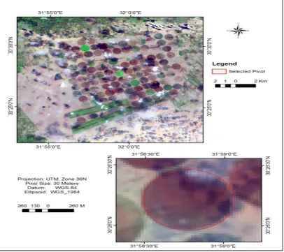
Site selectionAn irrigated pivot field in Sixths of October
Company for Agricultural Projects (SOAP) which located in El-Salhia Area, East of Nile Delta, Egypt was selected for soil salinity modeling (Fig. 1). It is bounded by 31º 58' 30" and 31º 59' 05'' longitudes and 30º 25' 55" and 30º 26' 30"
latitudes with a total area of 154 feddan.
Electromagnetic survey and analyses
The apparent soil conductivity (ECa) of the
pivot field was measured using Electromagnetic Induction (EM38) sensor (Geonics Ltd.,
Mississauga, Ontario, Canada) in millisiemens per meter (mS/m) at each coil separation In-phase response in parts per thousand (ppt) of secondary to
primary magnetic field at each coil separation before
wheat planted. A number of 432 EM38 survey readings were measured vertically and horizontally along 10 transects grid across the pivot study area with 90 meters averaged distance between each transect. The readings were performed few days before tillage and planting and after an irrigation event where the soil water content was close to the
field capacity. The maximum normalized residual
test was applied to EM38 signal data for outlier’s existence (Iglewicz and Hoaglin, 1993).
Soil sampling and analyses
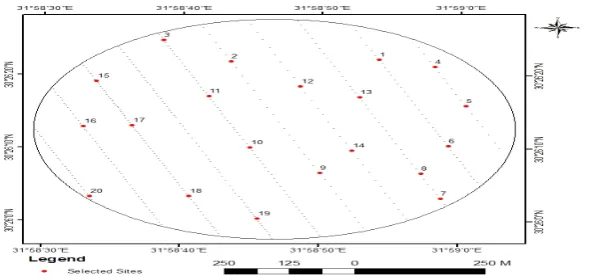
A spatial response surface design (SRS) (Corwin and lesch, 2005) was used to locate the best locations for soil sampling. Twenty soil sampling sites were located according to the selected SRS sampling design. Four soil variables were chosen for the selected SRS sampling sites which are soil salinity (ECe, dS/m), soil texture (clay, %), soil water content (WC, %), and soil organic matter (OM, %) at 30 cm depth intervals to a maximum depth of 90 cm (0-30, 30-60, and 60-90 cm). The soil samples were air-dried, crushed softly, and passed through a 2-mm sieve to get the
‘‘fine earth.’’ The fine earth was analyzed in the
laboratory according to (Soil Survey Staff, 2014).
Soil salinity calibration Modelling
A multiple linear calibration model (MLC)
was performed to predict the soil electric
conductivity levels within the pivot field using the
EM38 signal readings. The soil variable which has the most strength of the relationship against the standard variables (EM38 signal data (z1), the secondary (z2) EM38 signal data, and both the X and Y survey coordinates) was chosen as the soil variable for the model. The all possible model combinations were analyzed and the model with the lowest prediction errors was chosen as the more accurate model.
Soil salinity mapping
Interpolation between sampling locations was made by ordinary Kriging (Deutsch and Journel, 1992) interpolation method using ArcMap 10.2 (ESRI, 2013). Ordinary Kriging was used to estimate the value of a continuous characteristic z at a non-sampled locations (u) using only the
data on this characteristic [z (ua), α = 1, . . ., n] as
a linear combination of neighboring observations.
Results and Discussion
EM data descriptionThe obtained EM38 readings in the study pivot were subjected to descriptive statistical analyses. The statistical analyses results (Table 1) showed that, for the EM vertical readings (EMV) the data ranged between 12.00 and 333.00 with a mean of 64.35 and standard error of 2.79, also the lower
and upper bounds of 95% Confidence Interval for
Mean are 58.86 and 69.83 , respectively. While for the EM horizontal readings (EMh), the data ranged between 10.00 and 239.00 with a mean of 45.11 and standard error of 1.85, also the lower
and upper bounds of 95% Confidence Interval for
Mean are 41.48 and 48.75 , respectively. The data range for EMv and EMh readings was 321.00 and 229.00 , respectively. The results of variance are 3362.86 and 1479.46 for EMv and EMh readings respectively. Also, the standard deviation (SD) results are 57.99 and 38.46 for EMv and EMh readings , respectively. From percentiles and quartiles analyses, it appears that 50 % of EM readings lie between 12.00 and 36.50 for EMv readings and 10.00 and 28.00 for EMh readings, while 95 % of EM readings lie between 12.00 and 187.35 for EMv readings and 10.00 and 125.35 for EMh readings. The frequency distributions for EMv and EMh readings indicate that both vertical and horizontal EM readings follow nearly a
bell-shaped Gaussian distribution as about 84.72% and
85.65% of EMv and EMh readings , respectively lie within one standard deviation of the mean.
Soil variables
Four soil variables were chosen for the selected SRS sampling sites (Fig. 2). The considered soil variables are soil salinity (ECe, dS/m), soil texture (clay, %), soil water content (WC, %), and soil organic matter (OM, %) at 30 cm depth intervals to a maximum depth of 90 cm. The statistical analyses of the soil variables (Table 2) show that
the coefficients of variation (CV) of ECe were very high thus confirming the large variability
in soil salinity within the pivot. In contrast, the
coefficients variation of soil water content are the
lowest of the four variables.
Soil salinity calibration modeling
A multiple linear calibration model was performed to predict the soil salinity levels within
the pivot field using the EM38 survey readings
TABLE 1. Descriptive statistics of EM readings
Statistic Reading Statistic Reading
EMv EMh EMv EMh
Mean 64.35 45.11 Variance 3362.86 1479.46
Confidence -95% 58.86 41.48 Std.Dev. 57.99 38.46
Confidence +95% 69.83 48.75 Confidence SD -95% 54.36 36.06
Median 36.50 28.00 Confidence SD +95% 62.14 41.22
Minimum 12.00 10.00 Coef.Var. 90.12 85.26
Maximum 333.00 239.00 Standard Error 2.79 1.85
Skewness 1.90 2.05 Lower Quartile 26.00 20.00
Std.Err. Skewness 0.12 0.12 Upper Quartile 87.00 59.00
Kurtosis 3.87 4.93 Range 321.00 229.00
Std.Err. Kurtosis 0.23 0.23 Quartile Range 61.00 39.00
Fig.2. Selected SRS soil sampling sites
TABLE 2. Statistical analyses of the four soil variables
Soil
variable Depth
level Mean
std.
dev CV
% min max
Soil
variable Depth
level mean
std.
dev CV
% min max
ECe
30 1.617 1.811 112.00 0.21 5.98
WC
30 0.174 0.029 16.67 0.13 0.22
60 2.542 2.347 92.33 0.34 6.95 60 0.169 0.032 18.93 0.12 0.23
90 2.227 2.167 97.31 0.19 6.38 90 0.162 0.031 19.14 0.12 0.22
% Clay
30 11.588 4.497 38.81 5.15 19.15
OM
30 0.397 0.074 18.64 0.269 0.538
60 10.778 4.596 42.64 4.75 18.83 60 0.172 0.114 66.28 0.076 0.538
The results of the calibration model parameters combinations analyses indicated that, the Z1/Y parameters combination is the combination which produced the more accurate calibration model. The resulted calibration model for predicting soil
salinity within the pivot field using the EM38
conductivity survey readings is in the form :
ln (ECe) = b0 + b1(Z1) + b2(Y)
where :
ECe is the soil salinity,
Z1 and Y are the model variables and b0, b1, and b2 are model parameters
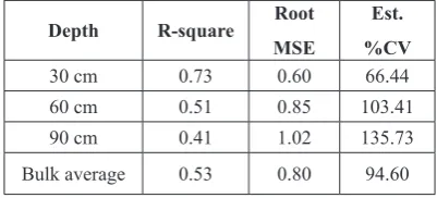
The calibration model was fitted to the bulk average, in addition to fitting to each set of depth
values. The calibration model summary statistics
for each fitted depth are shown in Table 4.
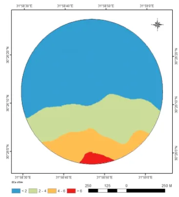
sampling locations for the specified sampling
depths by ordinary kriging interpolation technique. The spatial distribution of soil salinity for the
specified sampled soil depths are shown in Fig. 3.
Conclusions
The EM38 sensor provided non-invasive measurements of the apparent electrical conductivity (ECa) with less labor, cost and time intensive over other conductivity methods. The spatial response surface (SRS) sampling design allowed minimizing the number of samples required number of soil samplings to only a small set of 20 soil sampling sites to optimally estimate the spatially referenced regression model between the EM apparent electric conductivity (ECa) and the sampled soil electric conductivity. The sampled soil salinity correlated linearly with the EM signal data and indicated the incorporation of the trend surface parameters in the calibration modeling.
The multiple linear calibration (MLC) model
proved to be reliable for predicting the soil salinity
at the field scale for site-specific management.
Acknowledgement
The authors of this research acknowledge the Science and Technology Development Fund(STDF), Egypt for the financial support and also
acknowledge the Sixths of October Company for Agricultural Projects (SOAP) for the facilitation of conducting this research work. The authors also acknowledge the National Authority for Remote Sensing and Space Sciences (NARSS) for providing all the supporting material for this research work.
TABLE 3. Correlation coefficients between soil and regression variables
Soil variable Depth (cm) Z1 Z2 X Y
EC 3060 0.760.67 0.190.31 0.150.36 -0.85-0.71
90 0.60 0.07 0.10 -0.63
Clay 3060 0.600.51 0.120.15 0.420.42 -0.41-0.33
90 0.56 0.18 0.49 -0.43
WC 3060 0.660.56 0.100.17 0.370.39 -0.48-0.37
90 0.58 0.17 0.45 -0.44
OM 3060 -0.170.04 -0.310.20 -0.040.22 0.040.08
90 0.51 0.03 0.32 -0.36
TABLE 4. Calibration model Summary Statistics
Depth R-square Root
MSE
Est. %CV
30 cm 0.73 0.60 66.44
60 cm 0.51 0.85 103.41
90 cm 0.41 1.02 135.73
Bulk average 0.53 0.80 94.60
The R2 values of the calibration models for
the different soil sampling depths and the bulk average ranged between 0.41 for 90 cm soil depth and 0.73 for 30 cm soil depth. The R2 is being
significant at P< 0.001 for the 30 cm depth and significant at P< 0.01 for the remaining sampling
depths and bulk average. Thus, the calibration model accounted for 41% to 73% of the observed salinity variability at the different sampling depths.
References
Atwell M., Wuddivira M., Gobin J., and Robinson
D. (2013) Edaphic controls on sedge invasion in a tropical wetland assessed with electromagnetic induction. Soil Sci. Soc. Amer. J., 77, 1865-1874.
Bréchet L., Oatham M., Wuddivira M., and Robinson
D.A. (2012) Determining spatial variation in soil properties in teak and native tropical forest plots using electromagnetic induction. Vadose Zone J., 11, DOI:10.2136/vzj2011.0102.
Mapped soil salinity at 60 cm depth Mapped soil salinity at 30 cm depth
Mapped soil salinity at 90 cm depth Mapped soil salinity (bulk avarage) Fig. 3. Soil salinity maps at sampled depths
Corwin, D.L., and Lesch, S.M. (2005) Characterizing
soil spatial variability with apparent soil electrical conductivity. I. Survey protocols. Comput. Electron. Agric., 46, 103-134.
Deutsch, C. V. and Journel, A. G. (1992) GSLIB: Geostatistical Software Library and User's Guide.
Oxford University Press, New York.
G. and Zinck, J. A. (Ed.). Remote Sensing of Soil Salinization: Impact on Land Management. Taylor
and Francis Group, LIC.
ESRI(2013) ArcGIS Desktop: Release 10.2. Redlands,
CA, USA.
Haimelin R. (2008) Mapping soil water content on
agricultural fields using electromagnetic induction.
Report. Helsinki Universty of Technology, Helsinki. Iglewicz, B. and Hoaglin, DC. (1993) How to Detect and
Handle Outliers. Asqc Basic References in Quality Control, vol 16. American Society for Quality
Control.
Lesch, S. M. (2005) Sensor-directed surface response
sampling design for characterizing spatial variation in soil properties. Comp Electron. Agric.
Lund, E. D., Wolcott, M. C. and Hanson, G. P. (2001) Applying Nitrogen Site-Specifically Using
Conductivity Maps and Precision Agriculture Technology. 2nd International Nitrogen Conference
in Science and Policy. Potomac, MD, USA. Mann, K.K., Schumann, A.W., and Obreza, T.A. (2011)
Delineating productivity zones in a citrus grove using citrus production, tree growth and temporally stable soil data. Prec. Agri., 12, 457-472.
Martinez G., Vanderlinden K., Ordóñez R., and Muriel J.L. (2009) Can apparent electrical conductivity
improve the spatial characterization of soil organic carbon? Vadose Zone J., 8, 586-593.
McNeill, J.D. (1992) Rapid, accurate mapping of soil salinity by electromagnetic ground conductivity meters, Advances in Measurements of Soil Physics Properties: Bringing Theory into Practice, Soil Science Society of America Special Publication 30, American Society of Agronomy, Crop Science Society of America and Soil Science Society of America, Madison, Wisconsin, pp. 201–229 Moral, F.J., Terrón, J.M. and Silva, J.R. (2010)
Delineation of management zones using mobile measurements of soil apparent electrical conductivity and multivariate geostatistical techniques. Soil Till. Res. 106, 335-343.
Myers, R. H., and Montgomery, D. C. (2002) Response surface methodology: process and product optimization using designed experiments (2nd ed.).
New York, NY: Wiley.
Rhoades J.D. and Chanduvi F., (1999) Soil salinity assessment: Methods and interpretation of electrical conductivity measurements. FAO, 57, 1-150.
Rossi R., Amato M., Bitella G. and Bochicchio R.
(2013) Electrical resistivity tomography to delineate greenhouse soil variability. Int. Agrophys., 27, 211-218.
Soil Survey Staff (2014) Soil Survey Field and
Laboratory Methods Manual. Soil Survey
Investigations Report No. 51, Version 2.0. Manual, Natural Resources Conservation Service, U.S.
Triantafilis, J. and Lesch, S.M. (2005) Mapping clay
content variation using electromagnetic induction techniques. Comp. Elec. Agri. 46, 203-237.
Wuddivira, M.N., Robinson, D. A., Lebron, I., Bréchet L., Atwell, M., De Caires, S., Oatham, M., Jones ,
S.B., Abdu, H. Verma, A.K. and Tuller M. (2012) Estimation of soil clay content from hygroscopic water content measurements. Soil Sci. Soc. Am. J., 76, 1529-1535.
رصم – اتلدلا قرش ةقطنمب يسيطانغمورهكلا ثحلا مادختساب ةبرتلا ةحولم طيرخت
دمحم ديعس ديسلا و للاب بلطنملادبع للاب زيزعلادبع ، حلاص دعسم دمحا
رصم - ةرهاقلا - ءاضفلا مولعو دعب نع راعشتسلال ةيموقلا ةئيهلا - ىضارلأا مولع مسق
يوتسم يلع ةبرتلا ةحولم عيزوت ةطيرخ جاتنلا ىسيطنغمورهكلا ثحلا رعشتسم مادختسا وه ثحبلا نم فدهلا يلع دمتعت و حمقلا لوصحمب ةعورزم (توفيب) نادف 151 ةحاسم رايتخا مت. اهل ةقيقدلا ةرادلاا فدهب ةعرزملا ةجرد ريدقت مت ثيح اتلدلا قرش – ةيحلاصلا ةقطنم – ربوتكا نم سداسلا ةكرش يضاراب شرلاب يرلا تاينقت ةقطنمب عقوم 20 ديدحت مت. توفيبلاب عقوم 432 ددعب EM38 زاهج مادختساب ىرهاظلا يبرهكلا ليصوتلا كلذو ( spatial response surface sampling design(SRS)) ةيناكملا ةباجتسلاا جذومنل اقبط ةساردلا ةبسنو ةبرتلا ةحولم لثم صئاصخلا ضعب ليلحت فدهب مس 90 و 60 و 30 قامعا يلع ةبرتلا تانيع ذخلا . ةبوطرلا نم ةيرتلا يوتحمو ةيوضعلا ةداملا ةبسن و نيطلا