Xiao Wang
*, Dirk Burghardt
Dresden University of Technology, Institute of Cartography, [email protected], [email protected]
* Corresponding author
Abstract: Buildings are among the most important features of cities. In the suburban or rural regions, buildings are normally constructed along the roads, which forms the smooth and consistent patterns so that the building arrangements also can be described with network models. In previous studies, network theory has achieved good performance in cartography and GIS. In this paper, a study of a building-network is proposed, including the concepts, generation methods and centrality analysis. Firstly, with the constraint Delaunay triangulation and the refinement strategy by facing ratio, the building-network is generated by considering the buildings and the proximal segments as the nodes and segments of the network, respectively. Then, centrality analysis is applied on the building-network, aiming to reveal the crucial relationships among buildings, which is useful for understanding the structural properties of the complex network. Four different centrality measures, i.e. degree, closeness, betweenness, and eigenvector centrality, are calculated based on the building-networks. The buildings show different distribution effects and patterns under the four centrality measures. From the results, the degree centrality reveals the local centre of the region; closeness and eigenvector centrality have the ability to cluster buildings into different groups; while betweenness centrality can detect the linear patterns. Therefore, using network theory to analyse buildings can reveal some inner relationships of buildings and has great potential in the application of building pattern detection, classification, clustering and further generalization.
Keywords: building-network, network theory, centrality analysis
1. Introduction
In GIS, network data structures are one of the earliest representations, and network analysis remains one of the most important and persistent research areas (Curtin 2007). Previous research has shown that network analysis measures can be useful predictors for a number of interesting urban phenomena.
Network analysis or Graph Theory has already been applied in cartography for pattern detection and generalization (Mackaness et al., 1993). Particularly in road network, representations of road infrastructures as networks have been widely examined in the fields of GIS and network theory. Many studies have been carried out and achieved satisfying results. For example, the hierarchical structures of road networks can be formed with the network analysis (Zhang and Li, 2011). Graph theory is also introduced to solve the generalization problems of road network (Thomson and Richardson, 1995). With the centrality measures, the road network can be also analysed to investigate the characteristics of its representation and reveal the urban growth mechanisms (Crucitti et al., 2006) (Porta et al., 2006) (Lin and Ban 2017) (Lin and Ban, 2013). With the fruitful research achievements, the network analysis is supposed to have more potentials in analysing other geographical features. Therefore, the complex network theory provides a novel way to explore building features.
A city can be regarded as a complex network (Jiang 2016). As the two backbones of the city, roads and buildings are the most important features on maps. Buildings accommodate most urban activities and play as the crucial origins and destinations of urban movement. In the urban landscape, building plays an important role and correlates with urban development. In the real world, different regions show distinct distribution characteristics. In this sense, exploring buildings can reveal some underlying urban characteristics. However, unlike road network, which has the natural ability to become a network, the network property of buildings are always ignored for reasons of their unconnected distribution. It is so far fairly little in the spatial analysis of cities, specifically saying in urban buildings. The network analysis of urban buildings has been studied quite few. Previous study can be found in: Sevtsuk introduced an open-source Urban Network Analysis (UNA) toolbox, which computes five types of network centrality measures (Sevtsuk and Mekonnen, 2012).
measures and their application to the building-network. Section 4 discusses the centrality results. At last, the conclusion is given in Section 5.
2. Building-network
2.1 Concept of a building-network
There exist many networks in the world, virtual, physical, social etc. A network is a structure defined by nodes, and links between them. In geographical features, linear features have the natural ability to form a network because of their explicit connections, such as road network,
hydrographic network, and pipeline network1 (Figure
1(a)). The above mentioned geographical objects have the common features that they are all belong to one-dimensional linear feature type. With the specific connection relationships, linear objects are easy and natural to form the network.
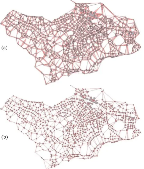
By contrast, building belongs to two-dimensional polygonal object in essence. Additionally, the connection relationships among buildings are mostly missing; thus, it is hard to regard buildings as a network apparently. Nevertheless, some buildings are represented with the linear patterns, which can be visually perceived with the network property (Figure 1(b)). Therefore, regarding buildings as the network is possible when there exist linear patterns within buildings.
Figure 1. (a) Road, pipeline, and hydrographic network; (b) Concept of a building-network.
1 Figures are derived from the websites:
https://www.gasnetworks.ie/corporate/company/our-network/pipeline-map/
https://www.eea.europa.eu/highlights/ecrins-map-project-pinpoints-water
2.2 Study area
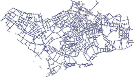
Because of population density, region functions and historical reasons, buildings are presented with different distribution features in different regions. As shown in Figure 2(a), in the central part of the cities, the buildings are normally distributed densely and adjacent with each other, which is hardly to be considered as having the network property. On the contrary, in the suburban or rural regions (Figure 2(b)), the buildings are mostly built along roads, which results in many linear building patterns. Linear patterns are smooth structures so that they can be perceived continuously in visual, which provides the potential for buildings to form a network.
Figure 2. Comparison between (a) city centre and (b) suburban region.
Based on the above descriptions, the network property is mainly represented in the suburban or rural regions of the city, where exists more residential areas than commercial or industrial areas. The buildings in residential area normally have the discrete distribution, simple shape and small size, which provides the possibility to generate a network. In our study, three villages around Dresden are selected as the test datasets, namely Weisser Hirsch, Pappritz, and Bühlau (Table 2). In the three selected villages, lots of obvious linear patterns can be found. These linear patterns create visual consistency on the discrete buildings so that the buildings can be perceived as network visually. The building number of the three village is 923, 744 and 1127, respectively. To generate the entire and complete network, the roads around the buildings are ignored in this study.
2.3 Generation of a building-network
Node and edge are two compulsory elements which should be determined to generate the network. The buildings are obviously the nodes of the building-network, here the centroids of the buildings are regarded as the nodes. The edges should be the connection relationships among buildings. Unlike road network, there are no explicit connection relationships among buildings, such that they should be founded firstly. The proximity graph is used to detect the neighboring buildings so that the connection relationship of buildings can be built (Zhang et al., 2013).
https://geoffboeing.com/2016/11/osmnx-python-street-networks/
(a)
(b)
Proximity graph is normally derived through constraint Delaunay triangulation (CDT). In this study, after getting the CDT, the triangles which connect three buildings should be deleted (Figure 3(a)); then each two buildings connected by the same triangle are detected as proximal so that their centroids are connected by a segment. The proximity graph is shown in Figure 4(b).
From Figure 3(b), although the connection
relationships have been built, it can be found that there exist many redundant proximal segments. For example, some buildings with distant positions are still connected, which violates the visual consistency. Therefore, the original proximity graph should be refined by removing these improper redundant connections. From the previous studies, many refinement methods have been proposed, such as Nearest Neighbour Graph (NNG), Minimum Spanning Tree (MST), Relative Neighbourhood Graph (RNG), Gabriel Graph (GG), and some parameters with Gestalt principles (such as distance, orientation, size, elongation, shape) (Anders 2003) (Yan et al., 2008). However, these refinement methods are mostly used for detecting building groups and recognizing patterns. The purpose of this study is to generate the building-network; thus, they cannot be directly used.
Figure 3. (a) CDT of buildings; (b) proximity graph of building.
To generate an entire and reasonable building-network, the facing ratio of two buildings is considered as the index to refine the original proximity graph. Facing ratio reflects the degree of two buildings that face with each other (Figure 4(a)) (Yang 2008) (Gong and Wu, 2018). The two buildings with a higher facing ratio indicates that they are more possible to be regarded as having the connection relationship. On the contrary, if the two buildings do not
face with each other, the connection should not be built between them.
The facing ratio between two buildings is calculated by Equation (1):
𝐹𝑎𝑐𝑖𝑛𝑔_𝑟𝑎𝑡𝑖𝑜 =𝑚𝑎𝑥𝑜𝑣𝑒𝑟𝑙𝑎𝑝(𝑃𝑟𝑜𝐿(𝐴), 𝑃𝑟𝑜𝐿(𝐵)) 𝑚𝑎𝑥(𝑃𝑟𝑜𝐿(𝐴), 𝑃𝑟𝑜𝐿(𝐵)) (1)
where ProL(A), ProL(B) denote the projection length of
building A and building B on the two axes of their
corresponding oriented bounding boxes. As shown in Figure 4(b), when calculating the facing ratio of two buildings, firstly, the oriented bounding boxes (OBB) of the buildings are derived; then, the OBBs are projected to their four axes; and the length on the axe is the projection length. The overlap rate of the projection length is calculated as their facing ratio in this axe. The maximum facing ratio of the four axes is regarded as the final facing ratio of these two buildings. If the facing ratio equals to 0, it means that the two buildings do not face with each other.
In the examples of Figure 4(b), Facing_ratioAC is 0.912,
Facing_ratioAB is 0.474, and facing_ratioBC is 0.0. Thus, it
concludes that building A faces with building B and
building C. Building B does not face with building C.
(a)
(b)
(a)
Building2 Building1
A B
C
Facing ratio
OA OB
OC YA
XB YB XA
XC YC Oriented bounding box
(b)
OB OA
Overlap1
Overlap2 YA
XA YB
XB
OB
OC YB
XB XC YC
OA
OC YC
YA X
A
XC Overlap1
Figure 4. (a) Facing ratio of buildings; (b) calculation of facing ratio.
In the refinement of the original proximity graph, if the facing ratio of two building is smaller than the given threshold; then, the proximal segments should be deleted from the proximity graph. The remained proximal segments will be the edges of the building-network.
2.4 Fine-tuning of facing ratio threshold
The refinement of the original proximity graph is important since it determines the final network. From the original proximity graph, it can be found that there are too many redundant segments. The refinement should eliminate the redundancy as much as possible, meanwhile, the completeness of the network should also be preserved as large as possible. Therefore, it is necessary to keep the balance between this two aspects.
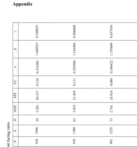
For this reason, different thresholds of facing ratio are selected to test the refinements effects. Taking the village Weisser Hirsch as example, the threshold of facing ratio is tuned from 0.0 to 0.4. When the facing ratio of the two buildings is smaller than the given threshold, the proximal edge will be deleted from them. When the threshold equals to 0.0, it means that if the buildings do not face with each other, the proximal edge will be deleted. The final generated building-networks with different facing ratio are listed in Table 1 in the appendix.
In the original proximity graph, there are 2005 edges in total. From the refinement results of different facing ratio thresholds, the refined proximity graph present the following characteristics: (1) with the threshold increasing, the nodes and edges of the network become decreasing; (2) The connectivity of the entire network becomes weaker and weaker. From Table 1, with the increasing thresholds, the buildings are divided into more and more network communities, so that the connectivity of the network becomes less and less. Connectivity reflects the connectedness within a network, which is a measure of accessibility without regard to distance. A high connectivity network denotes low isolation and high accessibility. The building-network should include buildings as much as possible, which is beneficial for generating an entire network.
The following network metrics in Table 2 are selected to measure the network properties in different thresholds.
Metrics Definition
Node (N) The number of nodes.
Edge (E) The number of edges.
Diameter (D) The longest shortest path joining
any two nodes in the network.
Average node degree (AND)
The average number of edges adjoining a node.
Average path length (APL)
The average shortest path length over the network.
Clustering coefficient (CC)
The average fraction of the node’s neighbours that are also neighbours with each other.
α
Characterizing the connectivity of a network between the observed number of cycles and the maximum number of cycles.
β Describing the complexity of a
network.
γ
Representing the ratio between observed number of edges and the maximum number of edges. It can measure how close the network is to complete.
Table 2. Metrics of describing network.
The values of AND, CC, α, β, γ are calculated by Equation
(2)-(6), respectively:
𝐴𝑁𝐷 =2𝐸
𝑁 (2)
𝐶𝐶 =1 𝑁∑
2𝑚𝑖
𝐶𝑖𝐷(𝐶 𝑖𝐷− 1) 𝑖∈𝑉
(3)
𝛼 =(𝐸 − 𝑁) + 1
2𝑁 − 5 (4)
𝛽 =𝐸
𝑁 (5)
𝛾 = 𝐸
3(𝑁 − 2) (6)
where mi indicates the number of edges between the first
neighbours of node i, CiD represents the degree centrality
of node I in the network.
Based on the definition, the metrics are calculated and listed in Table 1. From the statistics data in Table 1, with the facing ratio increasing, the generated building-network becomes more and more fragmented. Therefore, based on the above analysis, the facing ratio should be set tender, thus, setting as 0.0-0.2 should be the better option. In this study, we select 0.0 as the threshold. With the refined proximity graph, building-network is generated by regarding the buildings as nodes and the proximal segments as edges (Figure 5).
Figure 5. Final building-network (threshold = 0.0).
3. Centrality analysis of a building-network
3.1 Centrality measures
underlying topological mechanisms in the network. In this paper, four common centrality indices are adopted to analyse the importance of the building in urban building network, including degree centrality (DC), closeness centrality (CC), betweenness centrality (BC), and eigenvector centrality (EC).
3.1.1 Degree centrality
Degree centrality is a basic and simple index to measure the number of the connections between a given node and other nodes within the network. Degree centrality indicates that the important nodes in a network should connect to the other nodes as much as possible. The degree centrality is calculated as Equation (7):
𝐶𝑖𝐷= ∑ 𝑎
𝑖𝑗 𝑗∈𝑁
(7)
where N is the total number of the nodes; aij equals to 1 if
there is a connection between node i and node j, otherwise
it equals to 0.
3.1.2 Closeness centrality
Closeness centrality measures the shortest distance from a given node to all the other nodes, which shows how close the node is to the other nodes in the network. The more central a node is, the closer the node is to all the other nodes. The closeness centrality is calculated by the average length of the shortest path between the node all the other nodes in the network (Equation (8)):
𝐶𝑖𝐶= 1
𝐿𝑖
𝑁 − 1
∑𝑗∈𝑁;𝑗≠𝑖𝑑𝑖𝑗 (8)
where Li is the average distance from node i to all the other
nodes; N is the total number of nodes; dij is the shortest
distance between node i and node j.
3.1.3 Betweenness centrality
Betweenness centrality provides the means to quantify the likelihood a graph node will lie on a shortest path between two other nodes of the graph. It evaluates the number of shortest paths that pass through each node. Betweenness centrality measures the extent of a given node which is located between the paths that connects all other nodes. It quantifies the number of times a node acts as a bridge along the shortest path between two other nodes. In the graph, a node with a higher betweenness centrality value means that this node locates at the center position of the graph. The maximum betweenness centrality in a network specifies the proportion of shortest paths that pass through the most important node. The betweenness centrality of a
given node i can be calculated as (see Equation (9)):
𝐶𝑖𝐷= ∑ 𝑎
𝑖𝑗 𝑗∈𝑁
(9)
where N is the total number of nodes; njk is the number of
shortest paths from node j to node k, and njk(i) is the
number of shortest paths from node j to node k that pass
through node i.
3.1.4 Eigenvector centrality
Eigenvector centrality is a measure of the influence of a node in a network (Solá et al., 2013) (Iacobucci et al., 2017). It assigns relative scores to all nodes in the network
based on the concept that connections to high scoring nodes contribute more to the score of the node in question than equal connections to low scoring nodes. Eigenvector centrality shows. In the graph, a node is important if its
neighbours are important. For a given graph G=(N, E) with
N nodes and E edges. Let A=(ai,j) be the adjacency matrix,
i.e. ai,j=1 if node i is linked to node j, and ai,j=0 otherwise.
The eigenvector centrality score of node i can be defined
as (see Equation (10)):
𝐶𝑖𝐸=1
𝜆 ∑ 𝐶𝑗
𝐸
𝑗𝜖𝑀(𝑖)
=1
𝜆∑ 𝑎𝑖,𝑗𝐶𝑗
𝐸
𝑗𝜖𝐺
(10)
where M(i) is a set of the neighbours of i and λ is a
constant.
3.2 Centrality analysis
Based on the calculation metrics, the values of the above four centralities for every building in the three test villages
can be obtained. Buildings with different centrality values
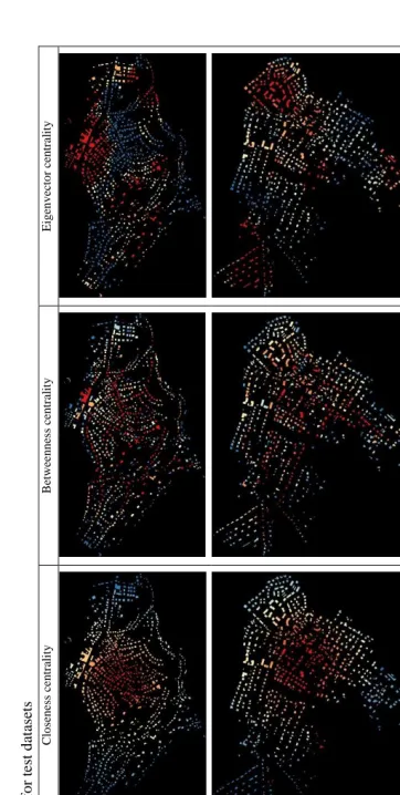
are displayed in different colours (Table 2). From the centrality results, the buildings present different patterns.
(1) Degree centrality is the most fundamental and straightforward measure to quantify the network’s connectivity. From the Table 2, the buildings which have large size, complex shape, or large elongation normally have the higher degree centrality values. These buildings with high degree values are important and can be regarded as the local centers.
(2) Closeness centrality reveals the level of travelling convenience of the nodes in a network, which can delineate the most accessible area of a network. From the distribution pattern, the buildings locate in the central area have the higher closeness centrality values while the buildings locate at the boundary area has the lower values. It presents the radial distribution, Therefore, based on the closeness centrality, it can differentiate the buildings located in the central or boundary areas.
(3) For betweenness centrality, it can measure the function of connectivity of a node in the network. The buildings which take part in forming the linear patterns normally have the higher betweenness values. These buildings are important in the building-network since they constitute the skeleton framework of the entire network.
(4) Eigenvector centrality reveals the importance of a node from another aspect. If a node connects with many other important nodes, it indicates that this node is also important in network. From the results of eigenvector centrality, the buildings present the clustering ability so that it can be used to form the building clusters.
From the above analysis of different centrality measures, the degree centrality focus more on the individual building while another three centrality consider the impact of other buildings. Specifically, betweenness centrality has beneficial for forming building alignments; closeness and eigenvector centrality have the ability to group buildings into different clusters.
4. Discussion
(1) Using network theory to analysis buildings, which provides a new way to reveal the inner relationships among buildings; (2) comparing with other methods (distance idea), the generation of the building-network considers the topology relationship to detect the neighbour relationships, which makes the network more consistency with the visual cognition; (3) the centrality analysis of building-network reveals the building patterns. The important buildings of the regions can be detected.
The shortage of the proposed method lies in that the buildings should have the discrete distribution; thus, the test datasets are derived from residential areas. For the buildings in the city centre, which have the obvious block distribution, the proposed method may have limitations.
The potential application fields of building-network can be located in building generalization. With the importance deriving from the centrality, the buildings can be classified so that it can provide the reference to the following generalization process. Meanwhile, with the centrality analysis results, other network techniques, such as network mesh, network Voronoi diagrams, can be widely applied into building-network.
5. Conclusion
This paper proposes the concept of building-network whereby the discrete buildings are connected in a network so that the network theory can be applied to analyse the building distribution. With the help of proximity graph and the refinement strategy by facing ration, the building-network can be generated. Through calculating the four centrality degrees, the buildings presents some regular patterns, which is beneficial for the further operations, such as local centre determination, building clustering and building generalization.
This study is the first step of introducing network theory to analyse urban buildings. The further step will be focused on using the network theory to achieve some specific application, such as building generalization.
Acknowledgements
This research was funded by German Research Foundation, grant number [DFG, BU 2605/5-1]. The first author also thanks to the support of Chinese Scholarship Council (CSC).
References
Anders, K. (2003). A hierarchical graph-clustering approach to find groups of objects. In Proceedings of the 7th ICA Workshop on Progress in Automated Map Generalization, April, 28-30th, 2003, Paris, France. Crucitti, P., Latora, V. and Porta, S. (2006). Centrality in
networks of urban streets. Pysical Review E, 73, 036125. Curtin, K.M. (2007). Network Analysis in Geographic
Information Science: Review, Assessment, and
Projections. Cartography and Geographic Information Science, 34(2), 103–111.
Gong, X. and Wu, F. (2018). A typification method for linear pattern in urban building generalisation. Geocarto International, 33(2), 189–207.
Iacobucci, D., McBride, R. and Popovich, D.L. (2017). Eigenvector centrality: Illustrations supporting the utility of extracting more than one eigenvector to obtain additional insights into networks and interdependent structures. Journal of Social Structure, 18(2), 1-22. Jiang, B. (2016). A City Is a Complex Network. In: M. W.
Mehaffy (editor, 2015), Christopher Alexander A City is Not a Tree: 50th Anniversary Edition, Sustasis Press: Portland, OR, 89-98.
Lin, J. and Ban, Y. (2017). Comparative Analysis on Topological Structures of Urban Street Networks. ISPRS International Journal of Geo-Information, 6(10), 295. Lin, J. and Ban, Y. (2013). Complex Network Topology of
Transportation Systems. Transport Reviews, 33(6), 658– 685.
Mackaness, W., Beard, K. and Hall, B. (1993). Use of Graph Theory to Support Map Generalization. Cartography, 210–221.
Porta, S., Crucitti, P. and Latora, V. (2006). The network analysis of urban streets: A dual approach. Physica A: Statistical Mechanics and its Applications, 369(2), 853– 866.
Sevtsuk, A. and Mekonnen, M. (2012). Urban network analysis: A new toolbox for ArcGIS. Revue internationale de géomatique, 22(2), 287–305.
Solá, L., Romance, Miguel., Criado, Regino., Flores, Julio., Garcia, A. and Boccaletti, S. (2013). Eigenvector centrality of nodes in multiplex networks. Chaos, 23(3). Thomson, R. and Richardson, D. (1995). A graph theory approach to road network generalisation. In Proceeding of the 17th International Cartographic Conference, September, 3-9, 1995, Barcelona, Spain, 1871–1880. Yan, H., Weibel, R. and Yang, B. (2008). A
multi-parameter approach to automated building grouping and generalization. GeoInformatica, 12(1), 73–89.
Yang, W. (2008). Identify building patterns. In Proceedings of the International Archives of the
Photogrammetry, Remote Sensing and Spatial
Information Sciences, Beijing, China, 3-11 July 2008; Volume XXXVII (Part B2), 391-397.
Zhang, H. and Li, Z. (2011). Weighted ego network for forming hierarchical structure of road networks. International Journal of Geographical Information Science, 25(2), 255–272.
Table
2.
Ce
ntr
al
it
y analy
sis of
urban b
uildin
g netw
ork for t
est
d
at
aset
s
Villag
e
Deg
ree
cen
tralit
y
Clo
sen
ess
centrality
Between
n
ess
centr
ality
Eigen
v
ecto
r
cent
ra
lity
W
eiss
er
Hirsch Pap
p
ritz
B
ü
h
lau
Lo
w