American Journal of Theoretical and Applied Statistics
2013; 2 (1) : 1-6Published online January 10, 2013 (http://www.sciencepublishinggroup.com/j/ajtas) doi: 10.11648/j.ajtas.20130201.11
Time series outlier analysis of tea price data
S. D. Krishnarani
Department of Statistics, Farook College, Kozhikode, Kerala, India
Email address:
krishna_manoharan@yahoo.com (S. D. Krishnarani)
To cite this article:
S. D. Krishnarani. Time Series Outlier Analysis of Tea Price Data. American Journal of Theoretical and Applied Statistics. Vol. 2, No. 1, 2013, pp. 1-6. doi: 10.11648/j.ajtas.20130201.11
Abstract:
In this article Autoregressive Integrated Moving Average (ARIMA) models were fitted and outliers are identi-fied for the auction price of tea in three regions- North India, South India and All India. The ARIMA models with seasonal differencing are found to be quite appropriate for the data. The region specific dynamics are distinctly assessed based on the autocorrelation functions. Further we are concerned with outliers in time series with two special cases, additive outlier (AO) and innovational outlier (IO).These outliers have been detected using two recent methods and conclusions drawn based on the data pertaining to the three regions. The reason for these types of outliers in the tea price have been further identified pointing towards the factors of environmental, weather conditions, pest attacks etc.Keywords:
Autoregressive Integrated Moving Average; Additive Outlier; Innovational Outlier; Tea Price Data1. Introduction
Time series observations are usually influenced by ab-normal observations which deviate significantly from the rest of the observations. Such observations are called out-liers. These outliers appear because of the unexpected or irregular events like weather conditions, strikes, economic instability, natural calamities and error in recording obser-vations. The outliers do affect the time series observations seriously, especially the autocorrelation function, partial autocorrelation function, model parameters etc. So they should be treated carefully. We mainly look into two types of outliers additive outliers (AO) and innovational outliers (IO). Additive outlier affects only a single observation and it is a result of a mistake made by a person in observation or record. But innovational outlier affects the subsequent observations starting from its position. The AO affects seriously the es-timates of the autoregressive moving average (ARMA) parameters, but the IO has less effect than AO. For more details about outliers see [1], [3], [4], [5], [7] etc.
Tea is one of the major agricultural commodities and India remains a major producer and exporter of tea worldwide. In India, tea production and exports of tea show a growing tendency for the last few years. The enormous fluctuations in the price of Indian Tea in the world market and quality deterioration of tea have become matters of concern for some time and these problems had already surfaced in the past years of the Indian Tea industry. The present paper seeks to throw fresh light on the recent trends of tea price in
India. Currently, India is the fourth largest tea exporting nation. The tea price in India has fluctuations although the general tendency is that of an increase over the years. One may refer to a recent report [9] which analyzed the tea price fluctuations in South India and North India using a second-ary data collected from tea statistics. The information we have from some reliable market source is that during 1990’s the average price of tea was not stable. In early 1990’s it was decreasing, in the mid 90’s there was a sudden increase and then a decline in the price. The price was lowest in 2001 compared with the price in late 90’s. But from 2002 it was increasing consistently. The price of almost all agricultural commodities has shown decrease in 1990’s. All these fluc-tuations may be mainly due to weather conditions, geo-graphical conditions, pest attacks etc. It is difficult to tify the variable effects and outliers. Our attempt is to iden-tify the outliers and the reason for these outliers. We have taken monthly data of tea price from the month of January 2006 to July 2011. We analyze the data and an ARIMA model with seasonal differencing is fitted and the outliers are identified.
2. Study Methods
residuals. Then we detected the presence of outliers in each data series through the procedure developed in [1] and [6]. Finally, we discussed each outlier in terms of management strategy and environmental influences.
Now we present the ARIMA models that we
paper. A useful class of time series model for modeling stationary data is autoregressive moving average models (ARMA) of the form,
) ( ) ( )
(B Xt θ B ε t
φ =
where
φ
(
B
)
andθ
(
B
)
are polynomials of degree p and q in B, the backward shift operator.But real time series data often exhibit some trend, which can be removed by taking differences. Such data is modeled using autoregressive integrated moving
order (p,d,q)(ARIMA(p,d,q)) having the general structure
) ( )
(B Xt dXt θ B ε
φ ∇ =
where ∇=1−B is the differencing operator, of order p, θ(B) is of order q and d is the order of di
Reference[1] generalized the ARIMA model to deal with seasonality and defined the model as
Q q t s P
pB B W θ B
φ( )Φ( ) = ( )Θ
where B denotes the backward shift operator,
, Φ , , Θ are polynomials of order p,P,q,Q respe
tively. t
D s d
t X
W =∇ ∇ denotes the differenced series. This model is called SARIMA model of order (p, d, q)(P, D, Q)s (See [2]).
Tea auction price data in three regions North India (NI), South India (SI) and All India (AI) are taken for study. data is taken from the website of Tea Board of section 2, we fit an ARIMA model with seasonal di
ing for the data. In section 3 outlier analysis of the same is done.
3. Time Series Analysis of Tea Price
Data
We analyze the tea price data of three regions, NI, SI and AI. We seek appropriate ARIMA model
Time series plot of the three types of data (Fig
that the data is not stationary, but shows an upward trend. To make the data stationary successive differences are taken to create new series. Now we look at the autocorrelation fun tion (ACF) and partial autocorrelation function (PACF) of the differenced series for determining the order of the most appropriate model.
The functions used in identifying model parameters are autocorrelation function (ACF) and partial autocorrelation function (PACF). First we analyze the data of NI. The time series plot shows non-stationary. For NI region the ACF (Figure 2) shows slight sine-cosine waves a
highly significant. PACF (Figure 3) is significant at lags 1, 5 residuals. Then we detected the presence of outliers in each data series through the procedure developed in [1] and [6]. Finally, we discussed each outlier in terms of management
the ARIMA models that we use in this paper. A useful class of time series model for modeling stationary data is autoregressive moving average models
(1)
are polynomials of degree p and
But real time series data often exhibit some trend, which can be removed by taking differences. Such data is modeled using autoregressive integrated moving average process of order (p,d,q)(ARIMA(p,d,q)) having the general structure,
) (t
ε (2)
erencing operator,
φ
(
B
)
is of order p, θ(B) is of order q and d is the order of difference. generalized the ARIMA model to deal witht s
Q(B)ε (3) where B denotes the backward shift operator, are polynomials of order p,P,q,Q
respec-denotes the differenced series. This model is called SARIMA model of order (p, d, q)(P, D, Q)s
ons North India (NI), are taken for study. The aken from the website of Tea Board of India. In MA model with seasonal differenc-ing for the data. In section 3 outlier analysis of the same is
Time Series Analysis of Tea Price
We analyze the tea price data of three regions, NI, SI and ARIMA models for these data. Time series plot of the three types of data (Figure 1) revealed that the data is not stationary, but shows an upward trend. To tionary successive differences are taken to create new series. Now we look at the autocorrelation func-tion (ACF) and partial autocorrelafunc-tion funcfunc-tion (PACF) of the differenced series for determining the order of the most
ed in identifying model parameters are autocorrelation function (ACF) and partial autocorrelation function (PACF). First we analyze the data of NI. The time stationary. For NI region the ACF cosine waves and each value is highly significant. PACF (Figure 3) is significant at lags 1, 5
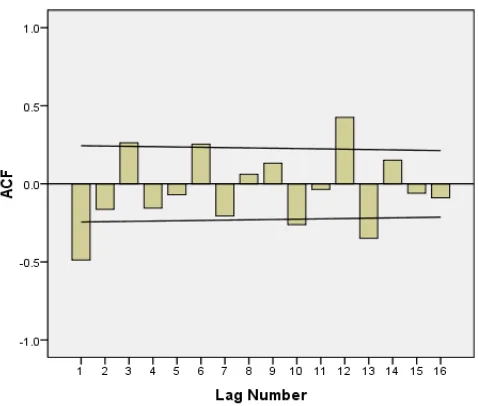
and 13. This shows that differencing is needed. After diff rencing the data by order 1, the ACF (Figure 4) and PACF (Figure 5) are plotted. The differenced data shows signif cant ACF at lags 1, 11, 12, 13 and 14 and PACF at 1,2,3,5 and 11. It is clear that an appropriate model can be ARIMA model or ARIMA model with seasonal component. The possible models are ARIMA(1, 0, 1), ARIMA(1, 0, 0)(1, 0, 0)12, ARIMA(1, 0, 0)(1, 0, 1)
and ARIMA(1, 0, 1)(1, 0, 1)12
(Table 1) are calculated for each model and it is minimum for ARIMA(1,0, 0)(1, 0, 0)12
and the PACF of the residuals (Figure 6) show that the va ues are within the given confidence intervals. The estimate of the model parameters are given in Table 2. Testing the significance of the model parameters is also done and the results are also shown in Table 2.
Figure 1. Time series plot of North India,
Figure 2. Sample auto-correlation function of N
and 13. This shows that differencing is needed. After diffe-rencing the data by order 1, the ACF (Figure 4) and PACF (Figure 5) are plotted. The differenced data shows
signifi-ant ACF at lags 1, 11, 12, 13 and 14 and PACF at 1,2,3,5 and 11. It is clear that an appropriate model can be ARIMA model or ARIMA model with seasonal component. The possible models are ARIMA(1, 0, 1), ARIMA(1, 0, 0)(1, 0, , ARIMA(1, 0, 0)(1, 0, 1)12, ARIMA(1, 0, 1)(1, 0, 0)12 12. The normalized BIC values (Table 1) are calculated for each model and it is minimum 12. The plot of the sample ACF and the PACF of the residuals (Figure 6) show that the val-ues are within the given confidence intervals. The estimate of the model parameters are given in Table 2. Testing the significance of the model parameters is also done and the results are also shown in Table 2.
Time series plot of North India, South India and All India regions.
American Journal of Theoretical and Applied Statistics 2013, 2 (1) : 1-6 3
Figure 3. Sample partial auto-correlation function of North India region.
Figure 4. Sample auto-correlation function of the differenced series of North India region.
Figure 5. Sample partial auto-correlation function of the differenced series of North India region.
Figure 6. Sample auto-correlation and partial auto-correlation function of the residuals of North India region.
Table 1. Normalized BIC values for the North India region.
Models BIC Values
ARIMA(1, 0, 1) 5.055
ARIMA(1, 0, 0)(1, 0, 0)12 4.685
ARIMA(1, 0, 0)(1, 0, 1)12 4.738
ARIMA(1, 0, 1)(1, 0, 0)12 4.762
ARIMA(1, 0, 1)(1, 0, 1)12 4.805
Table 2. Estimate of the model parameters for the North India region.
Type Estimate S.E t value p-value
Constant 89.288 15.548 5.743 0
AR(1) 0.851 0.064 13.39 0
SAR 0.653 0.116 5.260 0
The fitted model is
t t t
t
t X X X
X =89.288+0.851 −1−0.556 −12+0.653 −13+ε (4)
Table 3. Estimate of the model parameters for the South India region.
Type Estimate S.E t value p-value
Constant 62.965 7.919 7.951 0
AR(1) 0.946 0.036 26.034 0
Using the parameters, the estimated model is,
t t
t X
X =62.965 +0.946 −1 +ε .
Figure 7.Sample auto-correlation function of South India region.
Figure 8. Sample partial auto-correlation function of South India region.
Lastly we consider the AI data. The ACF (Figure 9) shows a wave-like pattern and PACF (Figure 10) significant at lags 1,2 and 13 which means that seasonal AR and MA terms are needed to model the data. First order differencing shows ACF (Figure 11) high at lag 3,6,12, but no clear pat-tern of PACF (Figure 12) suggesting that normal differenc-ing is not needed. So the possible models are ARIMA(1, 0, 1), ARIMA(1, 0, 0)(1, 0, 0)12, ARIMA(1, 0, 0)(1, 0, 1)12, ARIMA(1, 0, 1)(1, 0, 0)12, ARIMA(1, 0, 1)(1, 0, 1)12. The normalized BIC values (Table 4) are computed and it is shown that the suitable model is ARIMA(1, 0, 0)(1, 0, 0)12.
Also the sample ACF and sample PACF of the residuals support the suitability of the model.
Figure 9.Sample auto-correlation function of All India region.
Figure 10.Sample partial auto-correlation function of All India region.
American Journal of Theoretical and Applied Statistics 2013, 2 (1) : 1-6 5
Figure 12. Sample auto-correlation function of the differenced series of All India region.
Table 4. Normalized BIC values for the All India region.
Models BIC Values
ARIMA(1, 0, 1) 4.239
ARIMA(1, 0, 0)(1, 0, 0)12 4.031
ARIMA(1, 0, 0)(1, 0, 1)12 4.072
ARIMA(1, 0, 1)(1, 0, 0)12 4.067
ARIMA(1, 0, 1)(1, 0, 1)12 4.140
From the parameters (Table 5) we can form the model,
t t t
t
t X X X
X =80.66+0.91 −1− 0.5069 −12+0.557 −13+ε (5)
Table 5. Estimate of the model parameters for the All India region.
Type Estimate S.E t value p-value
Constant 80.66 14.18 5.7 0
AR(1) 0.91 0.05 18.266 0
SAR 0.557 0.119 4.671 0
The adequacy of fit of the models in the three cases is examined by considering the residuals as mentioned above. The estimated autocorrelation function and partial au-to-correlation function of the fitted models are within the upper and lower bounds.
The significance of the model parameters are tested using t- statistic. The modified L-jung Box Chi-square statistic is also used for testing the significance of residual sample autocorrelation functions with test statistic,
2 ∑ (6)
where is the residual autocorrelations. When n is large, Qk has a chi-square distribution with degrees of freedom k − p − q, where p and q are autoregressive and moving average orders, respectively. The significance level of Qk is
calcu-lated from the chi-square distribution with k- p - q degrees of freedom. The Box-Ljung statistic is defined in [8]. The value of the Ljung Box Chi-square statistic in the above three cases are given in Table 6.
Table 6. Ljung Box Chi-square statistic.
Region LBC d.f
NI 9.955 16
SI 6.704 17
AI 14.031 16
The values are not significant for the given degrees of freedom, and the corresponding models for the three data sets are accepted.
4. Outlier Analysis
This section mainly focuses on the additive and innova-tional outliers present in the data. The outliers in time series data severely affects the estimates of the model parameters and hence the model fitting. So it is necessary to have an idea about the presence of the outliers in the data. According to [1], an AO is modeled as
! (7)
where 1 if t=T and 0 if # $ %. An IO at time T is modeled as,
& '
( ' ) (8)
From this it is clear that AO affects the level of the ob-served time series only at time T, while IO affects the sub-sequent observations also. The presence of an outlier is tested using the likelihood ratio test criteria while the test statistics for IO and AO are respectively,
*, +-,,
./ and *0,
+-1,,
./ .
It is known that under the null hypothesis both follow standard Normal distribution. We have taken a critical value of 2.5 for this test. The detection of outliers is again verified with the method proposed in [6]. He has proposed a se-quential test, using the test statistic T* = maxTk*, where
) ,
max(1 2
*
k k
k T T
T = (9)
% 23 ∑ 452365 7 589
:. ;∑758945 <
(10)
and % 23
. (11)
The significance point is,
point k is additive otherwise innovational.
In the NI data four outliers are detected, additive outlier in March 2008 and Innovational outliers in April 2009,May 2009 and April 2011. For the SI region we could identify two outliers, innovational outliers in September 2008 and in December 2010. But in AI data innovational outliers come up in April 2009 and May 2009.
Now we examine the reasons for these types of outliers in the tea price. There is a decrease in production in the first three months of 2009 and this may be the reason for inno-vational outliers in 2009. As a result, a sudden increase can be seen in the price data. Also decrease in rain and severe drought conditions resulted in the outliers in the summer seasons like April, May 2009 and April 2011. Pest attacks and weather conditions also resulted a decrease in price in North India in 2009. Production in SI increased in Novem-ber 2010 and as an output an outlier can be seen in DecemNovem-ber 2010.In the AI region again outliers are present during the summer season of 2009.
The analysis we have done in the second section is under the assumption that no outlier is present in the data. Now we modify the model by considering the outliers and the model parameters are estimated. Table 7 reveals that there is not significant change in the model parameters before and after outlier detection. The residual sum of squares show a de-crease of 34%, 23% and17% respectively for the NI, SI and AI regions after identifying and adjusting outliers.
The model parameters after outlier detection are given in Table 7.
Table 7. Model parameters after outlier detection.
Region Type Parameter estimates Outliers
NI AR(1) 0.868 March 2008
MA(1) 0.019 April 2009
SAR(1) 0.899 May 2009
SMA(1) 0.208 April 2011
SI AR(1) 0.936 September 2008
December 2010
AI AR(1) 0.883 April 2009
SAR(1) 0.560 May 2009
5. Conclusion
In any statistical data analysis outlier has a major role in the model fitting and prediction processes. For the NI, SI and AI data we found that the most appropriate models are ARIMA(1, 0, 1)(1, 0, 1)12, ARIMA(1, 0, 0) and ARIMA(1, 1, 1)(1, 0, 0)12 respectively. The outliers were detected using two different methods proposed in [1] and [6]. In the
NI data four outliers are detected, additive outlier in March 2008 and Innovational outliers in April 2009, May 2009 and April 2011. For the SI region we could identify two outliers, innovational outliers in September 2008 and December 2010. But in AI data innovational outliers come up in April 2009 and May 2009. The reasons for these types of outliers in the tea price are attributed to a decrease in production in the first three months of 2009 accounted for innovational outlier in 2009. As a result, a sudden increase can be seen in the price data. Also decrease in rain and drought conditions in April 2009 resulted in the outliers. Pest attacks and weather con-ditions also resulted a decrease in price in North India in 2009. Production in SI increased in November 2010 and as an output an outlier can be seen in December 2010. In the AI region again outliers are present during the summer season of 2009.
Acknowledgement
The author would like to thank the anonymous reviewer and the editorial team for their constructive criticism and suggestions on an earlier version of this manuscript which led to this improved version.
References
[1] Box, G. E. P., Jenkins, G. M. and Reinsel, G. C., Time Series Analysis Forecasting and Control,3rd Edition, Pearson Education, Inc., 2009.
[2] Brockwell, P.J. and Davis, R. A., Introduction to Time Series and Forecasting,2nd Edition, Springer-Verlag, New York, Inc., 2006.
[3] Chatfield, C. , The Analysis of Time Series: An Introduction, 6th Edition, CRC Press LIC, 2009.
[4] Fox, A. J., Outliers in time series, J. Roy. Statist. Soc., B34, 350-363, 1972.
[5] Farley, E. V. , Jr. and Murphy, J. M. . Time series outlier analysis: Evidence for Management and Environmental In-fluences on Sockeye Salmon Catches in Alaska and Northern British Columbia, Alaska Fishery Research Bulletin, Vol.4, No.1, 1997.
[6] Louni, H. , Outlier detection in ARMA models, Journal of time series analy-sis., Vol.29,No.6,1057-1065, 2008.
[7] Kaya, A. , Statistical Modelling for Outlier Factors, Ozean Journal of Applied Sciences, 3 (no.1), 185-194. 2010.
[8] Ljung, G. M. and Box, G.E.P., On a measure of lack of fit in time series models, Biometrika, 65, 297-303, 1978.