Estimation Using Quantized Innovations for Wireless Sensor Networks

(1)

Estimation using Quantized

Innovations for Wireless

Sensor Networks

Noele Norris

Electrical Engineering, 2010

Minor in Control and Dynamical Systems

California Institute of Technology

Mentor: Babak Hassibi

(2)

2

Acknowledgements

I

would like to thank Babak Hassibi, my mentor who was always around to give valuable suggestions—for both my project and my academic endeavours, and Ravi Teja Sukhavasi, my brilliant grad-student mentor who kindly took me under his wing and who always took the time to explain and derive important concepts for me. I have learned so much under both of their guidance.

(3)

3

Abstract

(4)

4

Table of Figures

Figure 1: KLPF Simulation Plot. ... 10

Figure 2: Minero’s adaptive, exponential quantizer. ... 12

Figure 3: Minero Simulations ... 14

Figure 4: Yuksel Simulation ... 16

Figure 5: Probability distribution of state for KLPF ... 20

Figure 6: Simulation of KLPF in which error is higher than the SOI-KF Ricatti. ... 21

Figure 7: Simulation of KLPF in which error is lower than the SOI-KF Ricatti ... 22

Figure 8: Comparison of Minero and Yuksel with no Erasures.. ... 24

Figure 9: Comparison of Minero and Yuksel with no Erasures with no averaging.. ... 25

(6)

6

Introduction

Wireless sensor networks (WSNs) are networks of distributed, independent devices that monitor various environments or objects and wirelessly transmit measurements to a central base that can evaluate the information. They have become an increasingly popular technology and active field of interest not only because of the many interdisciplinary advancements that are making efficient and inexpensive ones possible but also because of their potential applications in diverse areas. The advancements made in integrated small-scale micro-electromechanical systems that have low power consumption pave the way for smart environments, "physical world[s] that [are] richly and invisibly interwoven with sensors, actuators, displays, and computational elements, embedded seamlessly in the everyday objects of our lives, and connected through a continuous network."1 In particular, WSNs can be used to monitor the ecosystem of a Redwood tree or monitor material responses to various vibrations and stresses,2 to track a vehicle or survey traffic flow, and even to track chemicals or make medical diagnostics.

WSNs have many advantages. As the sensors composing a network are usually distributed in large quantities, there is great robustness to sensor failure because of redundancies. There are also possible improvements in signal-to-noise ratios because of the network’s ability to reduce the distance between the sensors and their targets. Finally, the distribution of sensors across an environment creates the possibility of ‘multi-hopping’ transmissions over multiple nodes to a central base, which reduces required energy. However, the very benefits of WSNs create a number of challenges. Not only does the large distribution of sensors create design challenges because of the necessity of controlling a large number of independent devices, the small sensors have limited energy and communication capabilities as well as a limited ability to both process and store data.3

Thus, a great amount of research is currently being conducted to address both the various complexities and constraints of WSNs. One area of research tackles the particular challenge of energy and communication costs by considering the specific problem of tracking a noisy dynamical system (such as the position of a moving object) using discretized measurements from a number of sensors assuming that, at one measurement step, one sensor transmits only a constrained number of bits of information.

While the Kalman filter is the optimal estimator for a Gaussian system, constraining the measurements to a few bits creates nonlinearities that skew the probability distribution of the system so that the Gaussian assumption can no longer be assumed. Thus, the focus of this research was to design and analyze new methods of filtering for systems using quantized measurements. After analyzing an optimal particle filter designed by Sukhavasi ([3]) that uses the sign-of-innovation as the quantized measurement, various techniques were used to try to show that a linear dynamic system under sign-of-innovation measurements can be sufficiently tracked.

To do this, we first attempted to derive a recursive state estimation that used a

probabilistic set-membership description of uncertainty that probabilistically bounds the noises

1_{Mark Weiser quoted in [1]} _{D. Cook and S. Das,}

Smart Environments : Technology, Protocols and Applications. New York: Wiley-Interscience, 2004.

2_{These two applications are discussed in detail in [2]} _{F. Zhao and L. J. Guibas,}

Wireless Sensor Networks : An Information Processing Approach. Greensboro: Morgan Kaufmann, 2004.

(7)

7

(8)

8

Discussion and Results

Developing an Estimator for a Wireless Sensor Network

Quantizing the Measurement using the Sign-of-Innovation

The Kalman filter was developed in the 1960s and is a ubiquitous method of state estimation for a linear dynamic system in which both the noise and the conditional probability distributions of the states given the measurements are Gaussian. It is a recursive, minimum mean-square-error estimator that has the form of a linear observer, in which the observer gains are computed from error covariance matrices that are in turn calculated from a Riccati recursion equation (a type of difference equation). Kalman filters are popular because, not only are they optimal for Gaussian systems, they are computationally efficient and easy to implement. However, the Kalman filter cannot be used to track systems using severely constrained wireless sensor networks for a number of reasons. For one, under measurement quantization, the required Gaussian assumption no longer holds. More importantly, because the sensors are distributed, there is no central observer that has access to all of the full measurements so not even an observer can calculate the Kalman filter estimate—as has been done in other work on communication constrained control systems.

However, we can still use some of the principles used to develop the Kalman filter for a WSN. The Kalman filter is based on what is called the innovations process, which is the process of the error—the difference between the most current measurement and the controller’s estimate of what that measurement should have been given all previous measurements. The innovations process is a white process and can be “regarded as the ‘new information’ or the ‘innovation’ in the observation after we remove all we can say … about it from knowledge of past observations.”4 In [5], Ribeiro et al. used this concept for WSNs by assuming that all the sensors

can receive the controller’s estimate information (thus, assuming that it requires less energy to receive than to transmit), so that, in the case of using a communication channel with a one bit rate, the one bit of information that is transmitted from the sensor is the sign of the innovation (SOI) from its new measurement.

However, using the SOI, Ribeiro et al. incorrectly assumed that the conditional

probability density function of the state given the quantized measurement approximately follows

a normal distribution and, thus, proceeded to develop a modified Kalman filter (the SOI-KF) with a corresponding modified Riccati recursion which varies from the original Kalman filter Riccati only by a 2/π factor in front of the gain term, which accounts for the degree of quantization of the measurement.

Though Ribeiro et al. presented simulations of a couple of systems in which the SOI-KF seems to work, later work done by Sukhavasi has shown that their filter fails and has diverging

error performance under many different systems.5

4_{From [4] T. Kailath}

, et al., Linear Estimation. Upper Saddle River, NJ: Prentice Hall, 2000.

5_{Sukhavasi did this using a general particle filter as explained in his paper [6] R. T. Sukhavasi and B. Hassibi,}

(9)

9

The Kalman-Like Particle Filter

As a result, Sukhavasi developed another filter presented in [3], called the Kalman-Like Particle Filter (KLPF). The particle filter is used when the assumptions of the Kalman filter cannot be met. Instead of assuming a normal distribution, the particle filter represents a belief of a state in a nonparametric form by a set of randomly selected state samples. Each sample is called a particle and is essentially a single hypothesis about what the true state may be. An ‘importance factor’ gives a particular weight to each sample, representing using Bayes’ rule the probability of the state given the measurements. The weights are then used in a resampling process that has a greater probability of keeping particles with more weight.

Though optimal in the case of non-linear and non-Gaussian systems, particle filters can be very computationally expensive because they can require a huge number of particles. However, Sukhavasi developed a variant of the particle filter that greatly reduced the number of particles needed to optimally run the filter by breaking the probability model of the system into two parts—one that could be described as a Gaussian distribution and the other which had to be evolved using a particle filter. He noted that the original state-space model (without the measurement quantization) follows the Gaussian assumptions necessary to use a Kalman filter, while the one-bit quantization of the measurements creates nonlinearities that must be addressed by other estimation techniques. Thus, each particle addresses the skewed probability of the original measurement given its quantization, and the Kalman filter evolves the state estimate using the various guesses of the original (un-quantized) measurement. Therefore, this filter effectively runs a Kalman filter on each particle, where each particle represents a possible value of the original measurement based on the quantized measurement that is received.

Simulating the KLPF with the SOI-KF

(10)

10

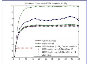
Figure 1: KLPF Simulation Plot. Plot of the evolution of the error of a particular dynamical system averaged over 50,000 iterations, each using a particle filter with 1000 particles

The Probabilistic Set-Membership Description

With the realization that there was no meaningful relationship between the SOI-KF Riccati and the evolution of the error of the KLPF, work shifted to trying to prove performance through a careful analysis of the original equations that described the system dynamics and quantized measurement updates. The performance of the KLPF could be verified if it could be shown that a marginally unstable system could be tracked with sufficiently bounded error when using only a sequence of bits, each representing the sign of the innovation.

To do this, an approach was tried that was inspired by work done by Schweppe and then Bertsekas in the late 60s ([7], [8]). Schweppe and Bertsekas derived recursive state estimations under a ‘set-membership description of uncertainty.’ The set-membership describes “input disturbances and observation errors [when they] are unknown except for the fact that they belong to given bounded sets.” [8] The sets they used were ellipsoids. They showed that intersecting ellipsoids, representing the bounds on the state both from the understanding of the state’s initial position and state evolution as well as from the measurement update, will result in an ellipsoid bounding the current state. This recursive process is not the best filter because the center of the resulting ellipsoid cannot be shown to be the optimal estimate of the state. However, if the ellipsoids remain bounded, it equivalently bounds the error in the estimate of the state of the system.

(11)

11

Thus, in this system, the noise could only be bounded probabilistically within ellipsoids, which

is equivalent to defining the variance of the noise using Gaussian confidence intervals.

Using Chernoff bounding techniques, a very similar recursive estimation process was developed for the probabilistic ellipsoids (shown in The Probabilistic Set-Membership Description, 22). With a recursion process at-hand, the goal became to show that, at each time step, an exponentially decaying probability bound held for the error measurement, which would then prove that the error covariance matrix remained bounded for all time. Using the state-dynamics equations, the probability bounds were evolved using the set-membership techniques to sum and intersect ellipsoids. Another main difference was that, instead of intersecting two ellipsoids to combine the bounds on the state based on its possible evolution from its initial position as well as from its measurement, in this case, the state-evolution ellipsoid could only be intersected with a half-plane that corresponded to the measurement bit received.

While this approach did give a method for evolving the probability bounds through time, the probability bound obtained at the end of a single recursion step was not tight enough to prove bounded error. Instead it had a very counterintuitive result, showing that the best estimate was obtained simply by evolving the mean estimate of the initial state and never using any of the quantized measurements. Thus, while simulations showed that the KLPF had bounded error, this technique could not verify it.

Literature Review

Because the probabilistic set-membership approach cannot be used to develop a tight recursion for the system, it has neither shown that the KLPF can be used to track a system nor that it cannot be used. Therefore, still needing to develop techniques to prove performance for the KPLF, we analyzed previous research that had instead created various coder-estimator pairs to prove stabilizability for closed-loop control systems under communication constraints. One result in this area of work on networked control systems that is especially applicable to our system is called the data-rate theorem and is inspired by Shannon’s source coding theorem. It states that, to stabilize a scalar system, the rate of the communication channel must be greater than the intrinsic entropy rate of the system, which is the logarithm of the magnitude of its

unstable pole:

| |

Quite simply, this means that, to keep a bound on the estimation of the state, the rate used to communicate measurements for the estimation must be larger than the rate at which the system is growing.

(12)

to the cu that the t

M

M a time-va correctly changes rates of c in block identicall

H stabilizab

where n

random v T non-erasu And, mo for This mea This mak probabili M a standar most inte of a quan adaptive, inverse s partition Figure rrent measur echniques pr Minero’s Da Minero’s form arying feedb y received by randomly ov consecutive

s of n cons

ly distributed His result is

bility is that

is again the variable rate The main dif ure system a ost important

1, by Jensen

ans that, with kes intuitive ity of having Minero prove rd property u erested in the ntizer and co

, exponentia square of the the region.

e 2: Minero’s qu

rement and t resented wou

ta-Rate Th

mulation is f back channel y the decode ver time. H

time steps, M secutive cha d process ac

that, for thi

e length of t , and λ is the fferences wit are that now tly, that stab n’s inequality

h n > 1, the

sense if we g a rate of ze

es the necess used in infor e paper’s tec oder-decoder al quantizer

e number of

uantizer is an a

the estimate uld also be a

eorem

for a system l. While M er without er However, bec Minero prop annel uses cross blocks. is particular the channel e eigenvalue

th this result w an expecta

bilizability d y ([11], Theo

2 necessary co

consider the ero over a ch

sity of this co rmation theo chnique of p r pair. To pr

that has a f levels, 22v,

daptive, expone

12 e from all pa

applicable to

m with Gauss inero assum rror, the rate cause we mi poses a scen and then v ” [9] r system, the

2 1

block in wh e (assumed to t and the da ation must b depends on n

orem 2.6.2)

2 ondition for e scenario in hannel block. ondition usin ory (See [11 proving suffi rove sufficie average quan , where v is

ential quantizer

assed quantiz o the KLPF.

sian disturba mes that all b e at which th ght expect s nario in whic aries accord

e necessary

1

hich the rat o be unstable ata-rate theor

e taken beca

n. As the fu

. stabilizabili n which n =

.

ng an entrop 1], Theorem iciency, whi ency, Minero ntization err s the numbe

r. Picture taken

zed measure

ances and un bits sent ove

he channel s some correla ch the rate “ ding to an

and sufficie

e remains c e) of the sca rem for the ause R is a unction

ity becomes 1000 and th

py-power ine 17.7.3). Ho ch is an exp o relies on th ror that dim r of bits tha

n from [12].

ements, we h

ncertainties u er the channe ends inform ation betwee “remains con

independent

ent conditio

constant, R i alar system.

scalar fixed random vari is co

harder to en here is a non

equality, wh owever, we plicit constru he property minishes like

(13)

13

He also relies on the ability to use multiple time steps to transmit information about a single measurement so that the decoder’s information about the measurement can be refined as much as necessary. This is done by using a fixed value  number of channel blocks (each with n channel

uses in which the rate R remains constant) to send information about one measurement. Therefore, every n steps (denoted by iterator j), the decoder receives the measurement update

and updates the estimator using vj bits, where

Hence, there is a tradeoff in selecting : the smaller  is, the more measurements are transmitted to the decoder with less delay, and the greater  is, the more the decoder can refine the value of a single measurement.

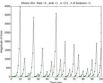
Simulations of Minero’s Algorithm

While Minero’s results did prove stabilizability for the system, we wanted to better understand the performance of the quantizer and encoder-decoder pair, so we simulated their algorithm on a number of various systems.

(14)

14

Figure 3: Minero Simulations. In the top simulation,  = 1. In the bottom simulation,  = 5.

0 10 20 30 40 50 60 70 80 90 100 0

0.5 1 1.5 2 2.5 3 3.5 4

Minero Sim: Rate =3 , prob =1 , a =2.5 , # of iterations =1

Time step

M

agni

tude of

E

rr

o

r

0 10 20 30 40 50 60 70 80 90 100 0

500 1000 1500 2000 2500 3000 3500 4000

Time step

M

a

gni

tu

de of

E

rr

o

(15)

15

Yuksel’s Stochastic Drift Result

Because Minero’s approaches used rather standard control-theoretic and information-theoretic techniques and also did not account for any possible channel erasures, we also analyzed Yuksel’s result in [10] for a stochastic communication channel that uses newer and what seem to be very powerful results from the theory of Markov chains on general spaces. Using notions of stochastic stability for Markov chains, Yuksel constructs a quantizer and encoder-decoder pair for estimating a state with measurements from a rate-constrained erasure channel and proves the filter’s stabilizability.

Like Minero’s work, Yuksel’s formulation is for a scalar dynamical system with unstable mode a, Gaussian noise disturbance, and Gaussian initial condition. While constraining the data

rate to R, Yuksel also allows for erasures of the form: 1

where 0 1 and 1 is the event that there is no erasure and that the signal is transmitted with no error at time step t.

Yuksel’s main result is that the necessary and sufficient condition for stabilizability of the plant is that

1

2 1 1

Notice that the result again follows the data-rate theorem: for p = 1, it reduces to the theorem and, for p = 0, the eigenvalue a must be stable.

(16)

16

Simulation of Yuksel’s Algorithm

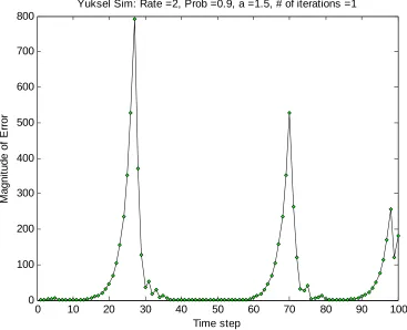
While Yuksel does prove stabilizability of his system, the biggest problem with it is that it does no more than that. Thus, even systems with values that well satisfy the sufficiency condition can produce very large estimation errors at particular time steps. An example simulation is shown below. (For more simulations, look at Minero and Yuksel Simulations, 23.)

Figure 4: Yuksel Simulation. Although the unstable mode only has a value of 1.5 and there is only a 0.1 probability of erasure, because the rate has been constrained to two bits, there are particular time instances with high estimation error.

However, although the algorithm is not of practical use, Yuksel’s result remains very important because it suggests new techniques for approaching the problem. Yuksel’s work shows that the general theory of Markov chains can be used as a powerful tool for understanding and deriving stochastic control systems.

0 10 20 30 40 50 60 70 80 90 100 0

100 200 300 400 500 600 700 800

Yuksel Sim: Rate =2, Prob =0.9, a =1.5, # of iterations =1

Time step

M

a

g

n

it

ude

of

E

rr

o

(17)

17

Markov Chains and Various Notions of Stochastic Stability

The last portion of our work has focused on better understanding the techniques used by Yuksel in [10] that are presented in Meyn and Tweedie [13]. Here is given a very brief introduction to Markov chains and some of the results and ideas presented in [13] that are most important to our current research.

First of all, a homogenous Markov chain is a particular type of random process that obeys the following very ‘nice,’ useful properties:

(1) Memoryless (Markov) property: The future state of the chain depends only on the current state of the chain and not on all its past states. Or more formally, the “conditional distribution of Xn+1 given (X0, …, Xn) depends only on Xn.” ([14])

(2) Time homogeneity: The conditional probability of a state given a particular value for the current state is the same for all time.

Examples of Markov chains include a random walk, a queuing system, and, of course, the state-space dynamical system that we have been analyzing. While the theory of Markov chains has existed since Markov’s pioneering work in the early 1900s, most of the work has focused on chains in countable spaces, that is, under the assumption that the state X can only take values from a countable set. Yet, this is clearly not the case for the Markov chain of the estimation error in our system. However, beginning in the 1950s with theories derived by Harris, it was shown that similar results could also be developed for chains on more general spaces. The theory of Markov chains on general spaces relies primarily on measure theory; instead of analyzing a collection of particular values of a countable set, we analyze sets of nonzero measure.

A Markov chain for a general space is defined by its transition probability kernel P(x, A), where, as defined by Meyn & Tweedie,

(i) For each A (X), P(·,A) is a non-negative measurable function on X and

(ii) For each x X, P(x, ·) is a probability measure on B(X)

where B(X) is a “countably generated” sigma field on X. A time-homogenous Markov chain Ф then satisfies the following equation for each n:

Ф , Ф , … , Ф … , … ,

where  is the initial distribution of the chain. (From [13], pages 59-61)

Meyn and Tweedie’s rigorous presentation of Markov chains is based on developing notions of stochastic stability. They write, “We will systematically develop a series of increasingly strong levels of communication and recurrence behavior within the state space of a Markov chain, which provide one unified framework within which we can discuss stability.” ([13], page 14) This communication that they refer to is the ability for the chain to reach, at some point in time, a set A of nonzero measure. This communication is described by requiring that the hitting time of set A is less than infinity:

inf 1 Ф

chain communicates with A: ∞

(18)

18

process. The weakest notion of stability in Meyn and Tweedie’s approach is thus that of ψ -irreducibility, which is the property that sets of nonzero measure (as measured by the function ψ) can be reached by the chain from every possible starting point:

, 0 ∞ 0

But, we want to ensure that not only is the set A visited, but that it is visited infinitely often, which is the property of recurrence and, because of the property of irreducible Markov chains, is equivalent to requiring that the set A is reached in finite time:

, 0 ∞

The strongest notion of stability that Meyn and Tweedie develop is ergodicity, which requires that the chain have “nice” limiting behavior in which its distribution converges to a limiting invariant distribution:

,

(19)

19

Conclusions

Although the Kalman-like Particle Filter (KLPF) exploits both the tractability of the Kalman filter and the optimality of particle filters and simulations have also shown good performance, we have still been unable to rigorously prove that it follows any performance specifications. However, in our attempts to prove stabilizability and other performance measures for the KLPF, we have determined that the optimal estimation error of a state under quantized measurements does not follow a Riccati-like recursion. We have also studied a number of results for control under communication constraints that have given us a toolbox of techniques and algorithms for approaching these problems.

While many of these techniques are founded on combining and modifying ideas and results from traditional information and control theories, Yuksel’s approach using Markov chains in [10] relies primarily on analyzing the probabilistic nature of the control system. This very general technique that uses the theory of stochastic stability offers great potential, and further work needs to be done to use these types of techniques to prove the performance of the KLPF.

(20)

Method

Problem T where x( w(n)~N(0 v(n)~N(0 using the under mu sensors, w the sign estimate O of the sys

where C i

The KLP

In [3]

ds

m Formulatio

The state-spa

(n) is the s 0,Q) and y( 0,R). While e measureme uch harsher where

of the inno of the measu Our primary

stem remain

is some consta

PF

], Sukhavasi

on and Sign

ace system be

state evolvin (n) is the m e the origin ents y1:n , the

conditions—

ovation of th urement give

goal is to de ns bounded fo

su ant.

i shows that

Figu

n of Innova

eing measur 1

ng under a measurement

al Kalman e goal of this —when the e

he measurem en all previo evise a filter for all time, o

up _N

the probabil

ure 5: Probabil

20

ations

red can be su

constant m t of the stat filter optima s research is estimator on

ment (the d ous measurem under these or that lity distributi lity distribution ummarized m

matrix A wit te also unde ally estimat s to show tha nly receives a

| 1

difference in ments).

conditions w

,

ion of the sy

n of state for KL

mathematica

th additive er additive G

es the filter at the system

a bit sequen

n the measu

which ensur

ystem is as fo

LPF

lly as

Gaussian n Gaussian no r by recursiv m can be trac nce b1:n from

urement and

res that the e

(21)

21

Thus, in the KLPF, the truncated normal distribution of y1:n | b1:n is estimated using a particle filter, while a Kalman filter evolves x(n)| y1:n for each particle {yi1:n }i=1, ..., N.

KLPF Simulations

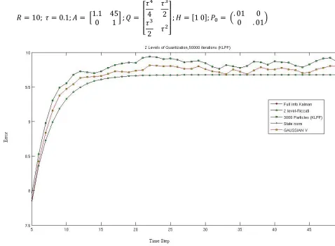
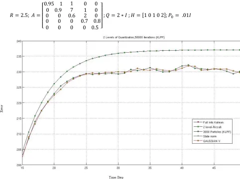
Using Monte Carlo simulations of the KLPF with 50,000 iterations each with 3,000 particles, systems were found in which the KLPF Riccati was above and below the SOI-KF Riccati. Therefore, it was concluded that the SOI-KF Riccati has no significance and does not characterize or bound the error of the optimal filter. (For more detailed descriptions of the KLPF and the SOI-KF refer to [3] and [5], respectively.):

 System 5: In system 5, the KLPF error is higher than that assumed by the SOI-KF Riccati.

10; 0.1; 1.1 45

0 1 ; 4 2

2

; 1 0 ; . 01 0

0 . 01

(22)

22

 System 12: However, in system 12, the KLPF has lower error than the SOI-KF.

2.5;

0.95 1 1 0 0

0 0.9 7 1 0

0 0 0

0 0₀

0.6 0 0

2 0 0.7 0.8

0 0.5

; 2 ; 1 0 1 0 2 ; .01

Figure 7: Simulation of KLPF in which error is lower than the SOI-KF Ricatti

The Probabilistic Set-Membership Description

If, for a multidimensional random variable X,

then its covariance matrix is finite (Appendix A.1). Thus, we want to recursively show that, at each time step, this exponentially decaying probability bound held for | .

The recursion evolved with the following initial conditions, which were proven using Chernoff bounding techniques on the original Gaussian noise assumptions:

0 0

(23)

23

where now, without loss of generality, x(0) ~ N(0, I) is the initial position of the k-dimensional state, v ~ N(0, σv2) is the measurement noise, and w ~ N(0,I) is the state evolution noise. Using the state-dynamics equations, the probability bounds on the state were evolved using the set-membership techniques to sum and intersect ellipsoids. The main difference is that instead of intersecting two ellipsoids to combine the bounds on the state based on its possible evolution from its initial position as well as from its measurement, the state-evolution ellipsoid was intersected with a half-plane that corresponded to the measurement bit, b(n), received.

In this manner (Appendix A.2), starting with a probability bound

| 1 | 1

after one step of the measurement update recursion the probability bound was

√ √ 1 1 1 2

where

| 1

√ 1

2

1 4

,

But here there are some problems. The ellipsoidal bound on the state | has a moving center; the center depends on n, which is simply the free variable that describes the probabilistically decaying bound. To prove a finite covariance, the center of the ellipsoid must be fixed. However, when trying to fix the center by any arbitrary shift corresponding to the bit received, the resulting covariance matrix is no smaller than if the estimate had not been updated based on the new measurement and was simply kept at the center at | 1 . Thus, this recursion does not track the system. Thus, this current analysis cannot be used to prove bounded estimation error because the bounds it creates are not tight enough to show that the error covariance remains finite.

Minero and Yuksel Simulations

Presented below are results from a few simulations of both Minero’s and Yuksel’s algorithms. The code used to run the simulations is presented in Appendix C: Minero Simulation Code, 30 and Appendix D: Yuksel Simulation Code, 35.

(24)

24

Comparison of Minero’s and Yuksel’s Algorithm with no Erasures Here results are averaged over 1000 iterations.

Figure 8: Comparison of Minero and Yuksel with no Erasures. In the top simulation of Minero’s algorithm, the minimum sufficient  of value two is used.

0 10 20 30 40 50 60 70 80 90 100 0

2 4 6 8 10 12 14 16 18

Minero Sim: Rate =3 , a =2.5 , # of iterations =1000

Time step

M

agni

tude of

A

v

er

age E

rr

o

r

0 10 20 30 40 50 60 70 80 90 100 0

50 100 150 200 250 300

Yuksel Sim: Rate =3, Prob =1, a =2.5, # of iterations =1000

Time Step

M

a

gni

tu

d

e

o

f

A

v

erag

e E

rr

o

(25)

25

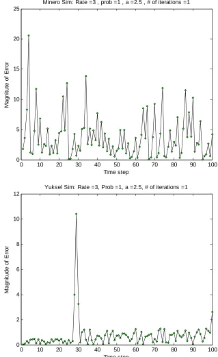
Comparision of Yuksel’s and Minero’s Algorithm with no Erasures: No Averaging

In the graphs below, only a single random iteration of the simulation was run. Thus, the averaging of Minero’s errors much more clearly shows when each measurement update was made (at every other time step, because of the choice of  = 2). For Yuksel’s simulation, notice that times of high estimation error occur infrequently over a single iteration.

Figure 9: Comparison of Minero and Yuksel with no Erasures with no averaging. In the top simulation of Minero’s algorithm, the minimum sufficient  of value two is used.

0 10 20 30 40 50 60 70 80 90 100 0

5 10 15 20 25

Time step

M

agni

tu

te

of

E

rr

o

r

0 10 20 30 40 50 60 70 80 90 100 0

2 4 6 8 10 12

Yuksel Sim: Rate =3, Prob =1, a =2.5, # of iterations =1

Time step

M

agni

tude of

E

rr

o

(26)

26

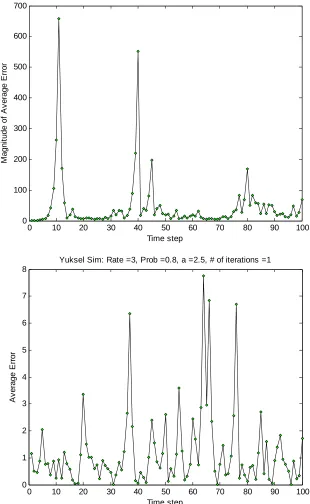
Comparing the effects of erasures on Yuksel’s simulation

Below are two graphs showing results from simulating Yuksel with a 0.2 probability of erasure. The first graph averages over 1000 iterations, while the second graph shows the outcome of a single iteration.

Figure 10: Yuksel simulation with 0.2 probability of erasure.

0 10 20 30 40 50 60 70 80 90 100 0

100 200 300 400 500 600 700

Time step

M

agn

it

ud

e of

A

v

era

ge E

rror

0 10 20 30 40 50 60 70 80 90 100 0

1 2 3 4 5 6 7 8

Time step

A

v

e

rage

E

rr

o

(27)

27

Appendices

Appendix A: Probabilistic Set-Membership Description Approach Lemma

If, for a multidimensional random variable X,

then its covariance matrix is finite.

This can be shown by writing Q-1 as a diagonal matrix: Since Q-1 is a real, symmetric matrix, it can be diagonalized by an orthogonal matrix A (ATA = AAT= I).

,

Since D is the diagonalization of a positive definite matrix, its eigenvalues are positive. Thus, for i = 1, ..., n,

We have thus reduced the problem to proving this for the one-dimensional case---that the variance of each yi is finite, as

For the one-dimensional case, we have:

1

Using this, we can easily show that is bounded.

Appendix B: Proabilistic Set-Membership Description Approach Recursion Attempt

Optimizing measurement update ellipsoid when y is scalar. Initial conditions:

| | √ Thus,

(1) scalar:

(28)

28 Measurement:

 b=1:

1 | | √

√ √ 1

& √ √ :

√

√ 1

 b=-1:

1

, 1:

√ 1

Thus, the general observation is:

(2) √ 1

Combining (1) and (2): 1

2 √

Measurement is useful if:

√ Assume that we are filtering:

Thus, the measurement is useful if: √

Since | 1 1| 1 , choose

3

Finally, we have:

√ Thus, the new ellipse is:

Radius:

√ 2

Mean:

√ 2

(29)

29 ;

This gives our new ellipsoidal bound:

2√ 1

1

4 1

We now need to intersect the original bound for x with the new bound from the measurement using a linear combination of the two bounds

1

1 0

0 0 1

2√ 1

1

4 1

1 2√ 1

2√ 1 4 1

1

1 4

Adding together:

1 2 √ 1

2 √ 1 4 1

1 1

4

Giving, after some algebraic manipulation:

2 √ 1 …

4 1

The bound can be rewritten as :

4 1

This gives us finally a bound of the form:

| | … 1 1

with

| | 1

2 √ 1

|

(30)

30

Appendix C: Minero Simulation Code

MineroSim.m

%Noele Norris

%Created: February 13, 2010 %Last Modified: April 29, 2010

%Simulate Coder-Decoder scheme in Minero's "Data Rate Theorem for %Stabilization Over Time-Varying Feedback Channels"

%Currently:only implementing for fixed rate; can only use with scalar %system though coding for vector system

%Also look at Nair's "Stabilizability of Stochastic Linear Systems with %Finite Feedback Data Rates"

%inputs to function: % R : fixed rate

% tau : number of channel uses for single measurement % p : rate of adaptive quantizer

% T : number of time steps % montecarlo : # of iterations

R = 3; tau = 5; p = 2; T = 100;

montecarlo = 1;

%System dynamics parameters

%Scalar system: x_k+1 = lam*x_k + u_k + v_k; y_k = x_k + w_k %unstable system: |lambda| >= 1

% A : system dynamics matrix

% Q : system disturbance covariance % H : measurement matrix

% sigv2 : measurement noise covariance % P_orig : covariance of initial state x_0

[A, Q, H, sigv2, P_orig] = System_params(); sigv2 = diag(sigv2);

sigv = sqrt(sigv2);

%Result: Mean square error

error_norm = zeros(1, T+1); error_norm_kf = zeros(1, T+1); state_norm = zeros(1, T+1);

%Kalman Riccati to be used in Kalman filter in coder %Computes estimate covariance P(k|k) and Kalman gain

HP_kalH = zeros(1, T+1); Kal_gain = zeros(1, T+1);

(31)

31

for i=1:T+1

%HP_kalH_quant(i) = diag(H*P_kal*H');

HP_kalH(i) = H^2*P_kal;

Kal_gain(i) = P_kal*H/(HP_kalH(i) + sigv2);

%P_kal - P_kal*H(j,:)'*H(j,:)*P_kal/(HP_kalH(j, i) + sigv2(j));

P_kal = (1 - Kal_gain(i)*H)*P_kal;

P_kal = A^2*P_kal + Q; %P(k+1|k) = AP(k|k)A^T + W(k)

end

%ITERATION

for iter = 1:montecarlo

iter

P = P_orig;

%measurement noise

V = normrnd(0, sigv, 1, T+1);

%initialize realization of state

X = zeros(1, T+1); mu_Xo = 0;

X(1) = mvnrnd(mu_Xo, P)'; %Initializing state; X0 ~ N(0, P)

%initialize realization of measurement

Y = zeros(1, T+1);

Z = zeros(1, T+1); %corresponding innovations

Y(1) = H*X(1) + V(1);

%initialize coder predictions (results of Kalman filter)

Xkal_hat = zeros(1, T+1); %coder's prediction of state hat{x}(k|k-1)

Xkal_updated = zeros(1, T+1); %coder's estimate of state hat{x}(k|k)

X_hat = zeros(1, T+1); %decoder's prediction of state

l = zeros(1, T+1); %scaling factor

l(1) = A^tau; %initialization of scaling factor

for t = 1:T+1

%time update: realization of state and measurement with coder's

%Kalman filtering update

if t == 1

Xkal_hat(t) = 0; X_hat(t) = 0;

else

u = -A*X_hat(t-1); %control input w/o quantization

(32)

32

Y(t) = H*X(t) + V(t);

%decoder's estimate

if mod(t-1, tau) == 0

%QUANTIZATION MEASUREMENT UPDATE

z = Xkal_updated(t-tau)-X_hat(t-tau); [k,q] = Quantizer(R*tau, p, z/l(t+1-tau)); X_hat(t) = pro(t)*A^(tau)*l(t+1-tau)*q; l(t+1) = max(l(1), k*l(t)*abs(A)^tau);

else

l(t+1) = l(t);

X_hat(t) = 0; %choose control input to bring state to zero

end

%measurement update

%calculate innovation

Z(t) = Y(t) -H*Xkal_hat(t);

Xkal_updated(t) = Xkal_hat(t) + Kal_gain(t)*Z(t);

end

error_norm = error_norm + sum((X - X_hat).^2, 1);

error_norm_kf = error_norm_kf + sum((X-Xkal_updated).^2,1); state_norm = state_norm + sum(X.^2, 1);

end

error_norm = sqrt(error_norm/montecarlo);

error_norm_kf = sqrt(error_norm_kf/montecarlo); state_norm = sqrt(state_norm/montecarlo);

time = 1:T;

figure;

plot(time, error_norm(1:T), '-kd','MarkerFaceColor', 'g', 'MarkerSize', 4); title(strcat('Rate = ', num2str(R), ' , prob =', num2str(prob), ' , a = ' , num2str(A) , ' , # of iterations = ' , num2str(montecarlo)));

Quantizer.m

%Noele Norris

%Created: February 13, 2010 %Last Modified: April 29, 2010

%Simulate Coder-Decoder scheme in Minero's "Data Rate Theorem for %Stabilization Over Time-Varying Feedback Channels"

%Currently:only implementing for fixed rate; can only use with scalar %system though coding for vector system

(33)

33

%inputs to function: % R : fixed rate

% tau : number of channel uses for single measurement % p : rate of adaptive quantizer

R = 3; tau = 5; p = 2; T = 100;

montecarlo = 1;

%Scalar system: x_k+1 = lam*x_k + u_k + v_k; y_k = x_k + w_k %unstable system: |lambda| >= 1

% A : system dynamics matrix

% Q : system disturbance covariance % H : measurement matrix

% sigv2 : measurement noise covariance % P_orig : covariance of initial state x_0

[A, Q, H, sigv2, P_orig] = System_params(); sigv2 = diag(sigv2);

sigv = sqrt(sigv2);

error_norm = zeros(1, T+1); error_norm_kf = zeros(1, T+1); state_norm = zeros(1, T+1);

%Kalman Riccati to be used in Kalman filter in coder %Computes estimate covariance P(k|k) and Kalman gain

HP_kalH = zeros(1, T+1); Kal_gain = zeros(1, T+1);

P_kal = P_orig;

for i=1:T+1

%HP_kalH_quant(i) = diag(H*P_kal*H');

HP_kalH(i) = H^2*P_kal;

Kal_gain(i) = P_kal*H/(HP_kalH(i) + sigv2);

%P_kal - P_kal*H(j,:)'*H(j,:)*P_kal/(HP_kalH(j, i) + sigv2(j));

P_kal = (1 - Kal_gain(i)*H)*P_kal;

P_kal = A^2*P_kal + Q; %P(k+1|k) = AP(k|k)A^T + W(k)

end

%ITERATION

(34)

34

iter

P = P_orig;

%measurement noise

V = normrnd(0, sigv, 1, T+1);

X = zeros(1, T+1); mu_Xo = 0;

X(1) = mvnrnd(mu_Xo, P)'; %Initializing state; X0 ~ N(0, P)

%initialize realization of measurement

Y = zeros(1, T+1);

Z = zeros(1, T+1); %corresponding innovations

Y(1) = H*X(1) + V(1);

%initialize coder predictions (results of Kalman filter)

Xkal_hat = zeros(1, T+1); %coder's prediction of state hat{x}(k|k-1)

Xkal_updated = zeros(1, T+1); %coder's estimate of state hat{x}(k|k)

X_hat = zeros(1, T+1); %decoder's prediction of state

l = zeros(1, T+1); %scaling factor

l(1) = A^tau; %initialization of scaling factor

for t = 1:T+1

%time update: realization of state and measurement with coder's

%Kalman filtering update

if t == 1

Xkal_hat(t) = 0; X_hat(t) = 0;

else

u = -A*X_hat(t-1); %control input w/o quantization

Xkal_hat(t) = A*Xkal_updated(t-1) + u; X(t) = A*X(t-1)+u + mvnrnd(0, Q)'; Y(t) = H*X(t) + V(t);

%decoder's estimate

if mod(t-1, tau) == 0

%QUANTIZATION MEASUREMENT UPDATE

z = Xkal_updated(t-tau)-X_hat(t-tau); [k,q] = Quantizer(R*tau, p, z/l(t+1-tau)); X_hat(t) = pro(t)*A^(tau)*l(t+1-tau)*q; l(t+1) = max(l(1), k*l(t)*abs(A)^tau);

else

l(t+1) = l(t);

X_hat(t) = 0; %choose control input to bring state to zero

end

(35)

35

%calculate innovation

Z(t) = Y(t) -H*Xkal_hat(t);

Xkal_updated(t) = Xkal_hat(t) + Kal_gain(t)*Z(t);

end

error_norm_kf = error_norm_kf + sum((X-Xkal_updated).^2,1); state_norm = state_norm + sum(X.^2, 1);

end

error_norm_kf = sqrt(error_norm_kf/montecarlo); state_norm = sqrt(state_norm/montecarlo);

time = 1:T;

figure;

plot(time, error_norm(1:T), '-kd','MarkerFaceColor', 'g', 'MarkerSize', 4); title(strcat('Rate = ', num2str(R), ' , prob =', num2str(prob), ' , a = ' , num2str(A) , ' , # of iterations = ' , num2str(montecarlo)));

Appendix D: Yuksel Simulation Code

YukselSim.m

%Noele Norris

%Created: February 23, 2010 %Modified: April 29, 2010

%Simulation of Yuksel's update rules in "A Random Time Stochastic Drift %Result and Application to Stochastic Stabilization over Noisy Channels" %inputs to function:

% p : probability that signal is transmitted with no error over 1 % channel use

% R: rate

T = 100;

montecarlo = 1;

count = 0; %number of instances error exceeds choosen value

%Scalar system: x_t+1 = a*x_t + u_t + d_t %unstable system: |a| >= 1

%Gaussian noise:

a = 2.5;

R = 3; %rate of transmission

prob = 0.8; %1 - prob = probability of erasure

(36)

36

P_orig = 1; %variance of x_0

K = 2^R;

R_p = log2(K-1);

%Values for determining quantizer bin size (look at Thm 3.2)

d = 0.05*abs(a); eta = 0.05*(K-1);

%%%

L = (K - 1 - eta)/abs(a); %threshold = 'L' in the paper

L_p = 1;

error_norm = zeros(1, T);

iter

X = zeros(1, T);

%vector of erasures

p = binornd(1, prob, [1 T]);

%initalization

del = zeros(1, T); %step size of adaptive quantizer

del(1) = 1;

X_hat = zeros(1, T); %decoder's prediction of state

X(1) = normrnd(0, P_orig);

for t = 2:T

Q_output = Quantizer(K-1, del(t-1), X(t-1));

if abs(abs(Q_output)-(K-1)*del(t-1)/2) < .0005

overflow = 1; X_hat(t-1) = 0;

else

overflow = 0;

X_hat(t-1) = p(t-1)*Q_output;

end

X(t) = a*(X(t-1)-X_hat(t-1)) + mvnrnd(0, Q); %state update,

with control input driving state to zero

%determine change in step size

if (p(t-1)== 0 || overflow == 1)

delMult = abs(a) + d;

elseif del(t-1) > L

delMult = abs(a)/(2^R_p - eta);

(37)

37

delMult = 1;

end

del(t) = del(t-1)*delMult;

end

if(max(X) >= 10^5)

count = count + 1;

end

time = 1:T;

count figure;

plot(time, error_norm(1:T), '-kd','MarkerFaceColor', 'g', 'MarkerSize', 4); title(strcat('Rate = ', num2str(R), ', Prob = ' , num2str(prob), ', a = ' , num2str(a), ', # of iterations = ' , num2str(montecarlo)));

Quantizer.m

function y = Quantizer(K, delta, x)

%is written only for odd K

if mod(K,2) == 0

error('K should be an odd positive integer'); end

y = zeros(size(x));

for i = 1:length(x)

if abs(x(i)) >= K*delta/2

y(i) = sign(x(i))*(K)*delta/2;

else

index = floor(2*abs(x(i))/delta); index_v2 = ceil(index/2);

y(i) = sign(x(i))*index_v2*delta;

end

(38)

38

References

[1] D. Cook and S. Das, Smart Environments : Technology, Protocols and Applications. New York:

Wiley-Interscience, 2004.

[2] F. Zhao and L. J. Guibas, Wireless Sensor Networks : An Information Processing Approach.

Greensboro: Morgan Kaufmann, 2004.

[3] R. T. Sukhavasi, "The Kalman Like Particle Filter : Optimal Estimation With Quantized Innovations/Measurements," presented at the 48th IEEE Conference on Decision and Control, Shanghai, China, 2009.

[4] T. Kailath, et al., Linear Estimation. Upper Saddle River, NJ: Prentice Hall, 2000.

[5] A. Ribeiro, et al., "SOI-KF: Distributed Kalman filtering with low-cost communications using the

sign of innovations," IEEE Transactions on Signal Processing, vol. 54, pp. 4782-4795, Dec 2006.

[6] R. T. Sukhavasi and B. Hassibi, "Particle filtering for Quantized Innovations," presented at the Proceedings of the 2009 IEEE International Conference on Acoustics, Speech and Signal Processing, 2009.

[7] F. C. Schweppe, "Recursive State Estimation - Unknown but Bounded Errors and System Inputs," IEEE Transactions on Automatic Control, vol. AC13, pp. 22-&, 1968.

[8] D. Bertsekas and I. B. Rhodes, "Recursive State Estimation for a Set-Membership Description of Uncertainty," IEEE Transactions on Automatic Control, vol. AC16, pp. 117-&, 1971.

[9] P. Minero, et al., "Data Rate Theorem for Stabilization Over Time-Varying Feedback Channels," IEEE Transactions on Automatic Control, vol. 54, pp. 243-255, 2009.

[10] S. Yuksel, "A Random Time Stochastic Drift Result and Application to Stochastic Stabilization Over Noisy Channels," presented at the Allerton Conference, Illinois, USA, 2009.

[11] T. M. Cover and J. A. Thomas, Elements of Information Theory, Second Edition ed. Hoboken,

NJ: Joyn Wiley & Sons, Inc., 2006.

[12] M. Franceschetti, "Data Rate Theorem for Stabilization over Time-Varying Feedback Channels: Workshop on Frontiers in Distributed Communication, Sensing and Control," ed, 2008.

[13] S. Meyn and R. L. Tweedie, Markov Chains and Stochastic Stability, Second Edition ed. New

York: Cambridge University Press, 2009.

[14] H. Olle, Finite Markov Chains and Algorithmic Applications. New York: Cambridge University