A fast iterative solver for scattering by elastic objects in layered media

A Fast Iterative Solver for Scattering by Elastic

Objects in Layered Media

K. Ito and J. Toivanen

Center for Research in Scientific Computation, North Carolina State University,

Raleigh, North Carolina 27695-8205

February 24, 2006

Abstract: We developed a fast iterative solver for computing time-harmonic acoustic waves scattered by an elastic object in layered media. The discretiza-tion of the problem was performed using a finite element method with linear elements based on a locally body-fitted uniform triangulation. We used a do-main decomposition preconditioner in the iterative solution of the resulting sys-tem of linear equations. The preconditioner was based on a cyclic reduction type fast direct solver. The solution procedure reduces GMRES iterates onto a sparse subspace which decreases the storage and computational requirements essentially. The numerical results demonstrate the effectiveness of the proposed approach for two-dimensional domains that are hundreds of wavelengths wide and require the solution of linear systems with several millions of unknowns.

1

Introduction

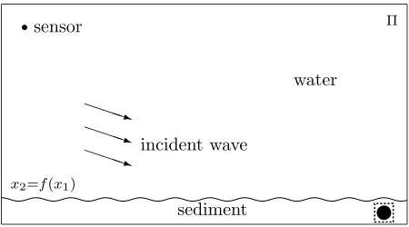
We consider a numerical method for computing time-harmonic acoustic waves scattered by an elastic object Ω in layered fluid. The proposed method is efficient when the interfaces between layers are nearly horizontal, for example, rippled horizontal interfaces. One application for such problems is the detection of hazardous or/and lost objects buried in sediment. For this purpose it is useful to have a numerical approximation which sufficiently accurately predicts backscatter by such targets.

x2=f(x1)

rsensor

water

sediment w

PPPq PPPq

PPPq incident wave

Π

Figure 1: A model problem with an elastic object Ω in sediment; the dashed line near Ω decomposes the domain Π into two subdomains which will be employed in the solution procedure.

fluid and for the displacementuin the elastic object Ω the partial differential equation model

∇ · 1 ρ∇p+

k2

ρ p=g in Π\Ω 1

ρ ∂p ∂n =ω

2_{u·n, −pn=σ(u)n on ∂Ω}

∇ ·σ(u) +ω2ρu= 0 in Ω Bp= 0 on∂Π,

(1.1)

whereω is the angular frequency, k =ω/c is the wave number,g is an acoustic source term, n denotes the unit outward normal vector of∂Ω, and σ(u) is the stress tensor. The operator B corresponds to a second-order absorbing boundary condition which is a generalization of the ones in [1, 7] for nonhomogenous media. For more discussion on scattering problems in layered media see [6], for example.

We discretize (1.1) using linear finite elements on uniform rectangular meshes which are locally adapted to the wavy sediment interface and the surface of the object. An algorithm to generate such meshes is described in [5], for example. In our solution procedure we employ a domain decomposition in which the near field subdomain is the interior of the dashed box in Figure 1 and the far field subdomain is the rest of the rectangle Π. For the second subdomain we construct a preconditioner based on a separable matrix obtained by discretizing perfectly vertically layered media without an object. Linear systems with such matrices can be solved efficiently using fast direct methods [29, 30, 34]. Since the media is vertically layered with a wavy interface, our preconditioner coincides with the system matrix except for the rows corresponding to unknowns near-by the interfaces. Due to this we can reduce iterations onto a small sparse subspace as has been shown in [19, 20]. This reduction makes our preconditioner much more efficient as our numerical examples demonstrate.

2

Finite Element Discretization

For two-dimensional problems, we use a generalization of the second-order absorbing bound-ary condition in [1] on the truncation boundbound-ary ∂Π, given by

1 ρ

∂p ∂n =i

k ρp+i

1 2k ∂ ∂s 1 ρ ∂p

∂s on∂Π 1

ρ ∂p ∂n =i

3k

4ρp at C,

(2.1)

where n and s denote the unit outward normal and tangent vectors, respectively, and C denotes the set of the corner points of ∂Π.

We construct a weak formulation by first multiplying the partial differential equations in (1.1) by test functionsq,v, and integrating the resulting equations over Π. We perform partial inte-gration in Π\Ω, Ω and apply the boundary/interface conditions in (1.1) and (2.1). After this¯ we perform partial integration along the four edges of Π and use the corner conditions in (2.1). This results in the weak formulation: Find (p, u) ∈ ©p∈H1(Π\Ω)¯ |p|∂Π∈H1(∂Π)ª ×

H1(Ω)d such that

Z

Π\Ω¯

1 ρ

¡

∇p·∇q−k2p q¢dx+

Z ∂Π i ρ µ 1 2k ∂p ∂s ∂q

∂s−k p q

¶

ds+ 3 4

X

C

1 ρp q

+

Z

∂Ω

¡

np·v+ω2u·nq¢ds+

Z

Ω

¡

σ(u) :²(v)−ω2ρ u·v¢dx=

Z

Π\Ω¯

g q dx

(2.2)

for all (q, v) ∈ ©q ∈H1(Π\Ω)¯ |q|∂Π∈H1(∂Π)

ª

× H1(Ω)d. We have used the notation σ(u) :²(v) = σij(u)²ij(v), where Einstein’s summation convention has been employed. The

stress tensor σ and the strain tensor ² are defined by

²(u) = 1

2(∇u+ (∇u)

We assume that the Lam´e constants µ and λ are constants on the elastic object. They are defined in terms of the compressional speed cc and the shear speedcs by

λ=ρ(c2c −2cs2) and µ=ρc2s.

Furthermore, we assume the wave number function k and the density function ρ to be piecewise constant.

We use linear finite elements based on meshes which are orthogonal and uniform except near the target Ω and the sediment interface where we locally adapt the meshes so that the boundary ∂Ω and the interface are approximated well. Such meshes can be generated fairly easily, for example, using the algorithm in [5]. A locally adapted mesh is shown in Figure 2. The meshes have to be sufficiently fine, say, at least 10 grid points per the wave length, so that they can approximate the oscillatory solution properly [18]. We use mass lumping leading to a diagonal mass matrix.

Figure 2: A part of a locally adapted mesh for the exterior of a circular target and a sinusoidal surface of sediment.

The discretization leads to the system of linear equations

Ax =b, (2.3)

where the matrix A has complex-valued entries and is non-Hermitian.

3

Iterative Solution

3.1

Domain Decomposition Method

We solve the system of linear equations (2.3) using the GMRES method [31] with a right preconditioner B leading to the system

AB−1y=b. (3.1)

The preconditionerB is based on the domain decomposition. In order to describe it we first express the matrix A in a block form

A =

µ

A11 A12

A21 A22

¶

, (3.2)

where the first block row corresponds to the near field subdomain inside the dashed box in Figure 1 and the second block row corresponds to the rest of Π. The vectors x and b have compatible block forms. Our preconditioner B has the upper block triangular form

B =

µ

A11 A12

0 S

¶

, (3.3)

where S = C22− C21C11−1C12 is the Schur complement of C11 in C which is described in

Section 3.2. The preconditioner B is of block Gauss-Seidel type.

Our choice of the preconditioner is motivated by the Neumann-Dirichlet domain decomposi-tion precondidecomposi-tioner; see [4, 33], for example. For a Poisson type equadecomposi-tion this precondidecomposi-tioner can be shown to be optimal in these sense that the condition number is bounded from above by a constant independent of the mesh step size. Our problem approaches such a problem when the frequency tends to zero. The matrix blockA11corresponds to a Dirichlet boundary

value problem in the near field subdomain. For the Poisson equation the Schur complement matrix S can be shown to be spectrally equivalent with a matrix resulting from a Neumann boundary value problem in the far field subdomain. Thus, the blockS can be considered to correspond to a Neumann boundary value problem. Based on these arguments we conclude that the preconditioner should lead to rapid convergence of the iterative method for low frequencies. It is not easy to analyze how rapidly the conditioning deteriorates when the frequency is increased. This behavior is studied in the numerical experiments in Section 4.

At each iteration a system of linear equations of the type

By=

µ

A11 A12

0 S

¶ µ

z1

z2

¶

=

µ

y1

y2

¶

=y (3.4)

needs to be solved. This can be performed in two steps:

1. Solve

C

µ

˜ z1

z2

¶

=

µ

0 y2

¶

(3.5)

using the fast direct method in Section 3.2.

2. Solve A11z1 = y1 −A12z2 using LU decomposition. Due to the small size of the near

3.2

System of linear equations with C

By discretizing the Helmholtz equation in the domain Π, without the object Ω and with a perfectly horizontal surface of the sediment, on a fully rectangular mesh we obtain a matrix

C=

µ

C11 C12

C21 C22

¶

, (3.6)

where the blocks correspond to our domain decomposition. Thus, the matrix block C11

corresponds to an acoustic scattering problem in the whole near field subdomain. The dimensions of blocks A11 and C11 are not the same, since A11 includes a part corresponding

to the elastic scatter Ω.

By renumbering the unknowns first from bottom to top (in the x2 direction) and then from

left to right (in the x1 direction) the matrix C has a tensor product form

C=H1⊗M2+M1⊗(H2−Mf2). (3.7)

The matricesH1 andH2correspond to stiffness matrices for one-dimensional problems in the

x1 andx2 direction, respectively, with special absorbing type boundary conditions. Similarly,

M1, M2, and Mf2 resemble scaled one-dimensional mass matrices which are diagonal due to

mass lumping. The dimension of the matricesH1 andM1 is the same as the number of nodes

in the x1 direction and they are given by

H1 =

1 h         

1−ihk/2 −1 −1 2 −1

−1 2 −1 . .. ... ...

−1 2 −1 −1 1−ihk/2

         and

M1 =h

        

1/2 +i/(2hk) 1

1 . ..

1

1/2 +i/(2hk)

         ,

where h denotes the mesh step size in the x1 and x2 direction. The matrices H2, M2, and

f

M2 can be considered to correspond to one-dimensional problems in the x2 direction and

their dimension is the number of nodes in thex2 direction. They can be assembled from the

elemental matrices He 2 = 1 hρe µ 1 −1 −1 1 ¶

, Me

2 = h 2ρe µ 1 0 0 1 ¶

, and Mfe

where ρe and ke are the density and the wave number on the one-dimensional element e in

the x2 direction. Due to the absorbing boundary condition the following additions have to

be made to these matrices: add −ik/(2ρ) into the first and last diagonal entry of H2, add

i/(2kρ) into the first and last diagonal entry of M2, and add ik/(2ρ) into the first and last

diagonal entry of Mf2.

Systems of linear equations with the matrix C can be solved efficiently using, for example, the cyclic reduction type fast direct solver considered in [15, 30]. The method is based on the diagonalization procedure: Let (Λi, Wi) be the eigen-pairs to the generalized eigenvalue problem

H1w=λ M1w.

Since H1 and M1 are symmetric, the eigenvectors are orthogonal with respect to the M1

-semi-inner product, that is,WTM1W =I. The properties of these eigenvalue problems have

been studied in [10]. If we let y= (W ⊗I)z then in the new variables C is diagonalized in the x1 direction, that is,

b

C = Λ1 ⊗M2 +I1⊗(H2−Mf2) (3.8)

is a block diagonal matrix with N1 diagonal blocks being tridiagonal matrices of dimension

N2. The direct transformation (W ⊗I)z and its inverse transformation are computationally

too expensive and there is no fast transformation like FFT available for the multiplication by the eigenvectors. Due to these reasons the cyclic reduction method is used for solving problems with C. For one solution this direct method requires O(NlogN) floating point operations [21, 30, 35], where N is the dimension of C.

3.3

Reduction to Sparse Subspace

We solve the right preconditioned system of linear equations given by (3.1) iteratively. For this a sparse subspace X is defined by

X = range(A−B) = range

µ

0 0

A21 A22−S

¶

. (3.9)

The jth component xj of an arbitrary vector x in X can be nonzero only if the jth row of

A and B do not coincide. Hence, the subspace X is called sparse. From the definition of X in (3.9), we see immediately that all vector components corresponding to the near field subdomain are zero inX. Due to the matrix blockA21the components corresponding to the

interface unknowns in the far field subdomain can be nonzero. Furthermore, components in the neighborhood of the interface between water and sediment can be nonzero due to the local adaptation of the mesh and non horizontal interface. Otherwise the components are zero corresponding to the interior of the far field subdomain. For the problems considered in this paper the dimension of X is very small compared to the size of the linear system (3.1). For the first test problem in Section 4.1 a sparse subspace is shown in Figure 3.

In the following, we consider iterative methods on the subspace X; see [19, 20] also. We let ˆ

y=y−b and then we have

where we have used the identity AB−1 =I+ (A−B)B−1. Furthermore, ˆy satisfies

£

I+ (A−B)B−1¤yˆ= ˆb (3.10)

and ˆy ∈ X. The reduced equation (3.10) is well suited for implementing the iterative procedure on the subspace X. If r ∈X then the Krylov subspace

span{r, AB−1r, · · · , (AB−1)k−1_}

is a subspace ofX. Thus, any iterative method based on the Krylov subspace for the solution of AB−1y=b generates a sequence of approximate solutions yk _{in the subspaceX provided}

that the initial iterate is y0 =b. Moreover, the basic operation

(A−B)B−1_{r, r ∈X}

which is repeated during the iterations requires the solutionsB−1ron the range of (A−B)T. The dimension of this range is the same order as the dimension of X. Due to this the systems of linear equations with C can solved using the partial solution technique [2, 23]. This technique is based on the observation that by taking advantage of the sparsity of vectors the transformation (W⊗I)z and its inverse transformation are computationally not too expensive and, thus, the diagonalization (3.8) can be used directly in the solution. For two-dimensional problems this reduces the computational cost of these solutions to beO(N) floating point operations, where N is the dimension of C.

In summary, the system of linear equations can be solved efficiently with the preconditioner B. The memory and computational requirements can be essentially decreased by reducing the GMRES iterations onto the sparse subspaceXdefined by the range ofA−B. Particularly, we can use the GMRES method without restarts which would usually severely degrade the convergence rate in this kind of scattering problems. This subspace corresponds to the interface between the subdomains and the neighborhood of the surface of the sediment where A and B differ.

4

Numerical Results

4.1

Scattering by a disk

We present numerical results on scattering by an aluminum disk with one feet diameter and the center at (0 m, −0.2524 m). The density of aluminum is 2700 kg/m3 and its compres-sional speed and shear speed arecc = 6568 m/s andcs= 3149 m/s, respectively. The surface

of the sediment is defined byx2 =f(x1) = (0.0368 m) cos(360◦x1/(0.75 m)). In the sediment

the density is 2000 kg/m3 and the speed of sound is (1668−16.8i) m/s, where the imaginary part attenuates waves. The density of water is 1000 kg/m3 _{and the speed of sound in it is}

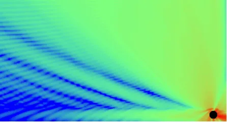
Figure 3: The sparse subspace X for the 561×305 mesh.

Figure 4: The intensity level of the scattered field for the frequency 8.056 kHz.

The sparse subspace for the coarsest mesh is depicted in Figure 4. The amplitude of the scattered field at 8.056 kHz is shown by Figure 4. In Table 1, f is the frequency in kHz, N gives the number of nodes in the mesh, and M is the dimension of the sparse subspace X. All times have been given in CPU seconds on a PC with an Intel Xeon 3.40 GHz and 2 GBytes of memory. The GMRES iterations were terminated when the norm of the residual was reduced by the factor 10−6. Based on the speed of sound in the sediment the width of the computational domain Π varies from 42 to 260 wavelengths.

Table 1 shows that the mesh step size does not have much influence on the number of iterations while the frequency does. Based on more extensive experiments than given in the table the number of iteration is roughly an affine function of the frequency which starts

f N M iter. time

8.056 561×305 2286 29 4

8.056 1121×609 6352 33 33 8.056 2241×1217 18979 30 255

19.564 1121×609 6352 53 48

19.564 2241×1217 18979 57 464 49.487 2241×1217 18979 95 733

¾

-1.3 m

¾0.65 m

-? 60.04 m ? 6

0.46 m

Figure 5: A crosscut of a Manta mine.

around 20 iterations for very low frequencies and then it grows about 1.5 iterations per one kHz. For frequencies above, say, 30 kHz methods based high frequency asymptotics are starting to be sufficiently accurate for many applications. The proposed method is especially efficient for problems below the frequency range of the asymptotic approximations.

4.2

Scattering by a crosscut of frustum

The second target is a crosscut of a Manta mine shown in Figure 5. Again the target is made of solid aluminum while a real Manta mine has complicated internal structure. The top of the target is 0.18 m below the mean level of the surface of the sediment which has the same shape as in Section 4.1. The properties of the materials are the same as in the previous problems. In this problem, we model a large computational domain given by Π = [−160 m, 160 m]×[−2 m, 60 m]. We have chosen the top boundary at x2 = 60 m to

be the interface between water and air. This leads to a homogenous Dirichlet boundary condition on this boundary.

A point sound source is located at (−150 m, 55 m) while in the x1 direction the target is in

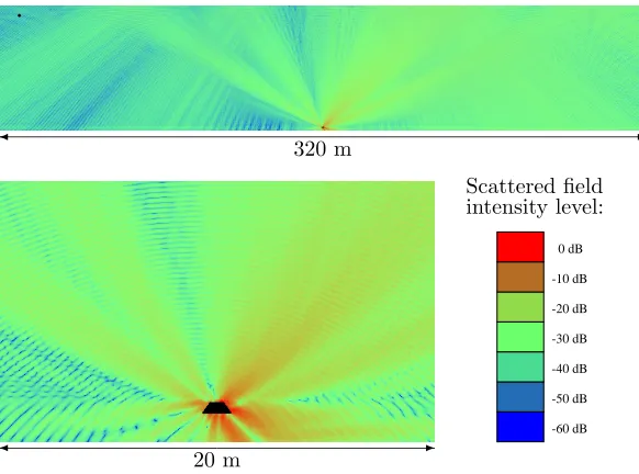
the middle of Π. Thus, the incident angle at the target is about 20◦. The frequency of the source is 3.15 kHz and, hence, the wavelength is about 0.48 m in water. Our mesh step size is 0.04 m which leads to a mesh with 8001×1551 nodes. The solution of resulting system of linear equations with about 12 million unknowns required 36 GMRES iterations and about 6 minutes. We have used the same computer and stopping criterion for the GMRES method as with the numerical results in Section 4.1. The dimension of the sparse subspace X was about 27500. The amplitude of the scattered wave is shown in Figure 6.

5

Conclusions and Future Research

¾

-320 m

¾

-20 m

-60 dB -50 dB -40 dB -30 dB -20 dB -10 dB 0 dB Scattered field intensity level:

Figure 6: The intensity level of the scattered field by the target in the whole computational domain Π (top) and near the target (bottom).

For more realistic problems, several generalizations have to be made. For example, we should consider a detailed model of the elastic object for practical target identification. The pro-posed method can be extended in a straightforward manner to three-dimensional problems. However, in order to develop a faster solver for three-dimensional domains further research is required. We remark that the wavenumber integration technique used, for example, by OASES [32] is not directly applicable due to interfaces which are not perfectly horizontal.

Here we mention some future research topics. In three-dimensional domains, the use of LU factorization in the solution of the problems in the near field domain can be computationally too expensive. Thus, a fairly effective iterative solution procedure is needed for near field problems. When there are many wavelength across the domain the phase error dominates the discretization error. By employing phase error reducing discretizations [11, 18] the same accuracy can be obtained by solving much smaller linear systems. The computational burden can be also reduced by developing a special FFT based fast direct solver for problems with absorbing boundary conditions and using this instead of the current cyclic reduction type fast direct solver.

Acknowledgements

References

[1] A. Bamberger, P. Joly, and J. E. Roberts, Second-order absorbing boundary

conditions for the wave equation: a solution for the corner problem, SIAM J. Numer. Anal., 27 (1990), pp. 323–352.

[2] A. Banegas,Fast Poisson solvers for problems with sparsity, Math. Comp., 32 (1978), pp. 441–446.

[3] H. T. Banks, K. Ito, G. M. Kepler, and J. A. Toivanen,Material surface design

to counter electromagnetic interrogation of targets, SIAM J. Appl. Math., (2006). To appear.

[4] P. E. Bjørstad and O. B. Widlund, Iterative methods for the solution of elliptic

problems on regions partitioned into substructures, SIAM J. Numer. Anal., 23 (1986), pp. 1097–1120.

[5] C. B¨orgers,A triangulation algorithm for fast elliptic solvers based on domain imbed-ding, SIAM J. Numer. Anal., 27 (1990), pp. 1187–1196.

[6] J. L. Buchanan, R. P. Gilbert, A. Wirgin, and Y. S. Xu, Marine acoustics:

Direct and inverse problems, SIAM, Philadelphia, 2004.

[7] B. Engquist and A. Majda, Absorbing boundary conditions for the numerical

sim-ulation of waves, Math. Comp., 31 (1977), pp. 629–651.

[8] Y. A. Erlangga, C. W. Oosterlee, and C. Vuik, A novel multigrid based

pre-conditioner for heterogeneous Helmholtz problems, SIAM J. Sci. Comput., (2006). To appear.

[9] Y. A. Erlangga, C. Vuik, and C. W. Oosterlee,On a class of preconditioners

for solving the Helmholtz equation, Appl. Numer. Math., 50 (2004), pp. 409–425.

[10] G. Fibich and S. Tsynkov, Numerical solution of the nonlinear Helmholtz equation

using nonorthogonal expansions, J. Comput. Phys., 210 (2005), pp. 183–224.

[11] M. N. Guddati and B. Yue, Modified integration rules for reducing dispersion in

finite element methods, Comput. Methods Appl. Mech. Engrg., 193 (2004), pp. 275– 287.

[12] E. Heikkola, Y. A. Kuznetsov, P. Neittaanm¨aki, and J. Toivanen,Fictitious

domain methods for the numerical solution of two-dimensional scattering problems, J. Comput. Phys., 145 (1998), pp. 89–109.

[13] E. Heikkola, T. Rossi, and J. Toivanen, A domain decomposition technique for

[14] , A domain embedding method for scattering problems with an absorbing boundary or a perfectly matched layer, J. Comput. Acoust., 11 (2003), pp. 159–174.

[15] , Fast direct solution of the Helmholtz equation with a perfectly matched layer/an absorbing boundary condition, Internat. J. Numer. Methods Engrg., 57 (2003), pp. 2007– 2025.

[16] , A parallel fictitious domain method for the three-dimensional Helmholtz equation, SIAM J. Sci. Comput., 24 (2003), pp. 1567–1588.

[17] Q. Huynh, K. Ito, and J. Toivanen, A fast Helmholtz solver for scattering by a

sound-soft target in sediment, in Proceedings of the 16th International Conference on Domain Decomposition Methods, 2006. To appear.

[18] F. Ihlenburg,Finite element analysis of acoustic scattering, vol. 132 of Applied Math-ematical Sciences, Springer-Verlag, New York, 1998.

[19] K. Ito and J. Toivanen,Preconditioned iterative methods on sparse subspaces, Appl.

Math. Letters, (2006). To appear.

[20] Y. A. Kuznetsov, Matrix iterative methods in subspaces, in Proceedings of the Inter-national Congress of Mathematicians, Vol. 1, 2 (Warsaw, 1983), Warsaw, 1984, PWN, pp. 1509–1521.

[21] , Numerical methods in subspaces, in Vychislitel’nye Processy i Sistemy II, G. I. Marchuk, ed., Nauka, Moscow, 1985, pp. 265–350. In Russian.

[22] Y. A. Kuznetsov and K. N. Lipnikov, 3D Helmholtz wave equation by fictitious

domain method, Russian J. Numer. Anal. Math. Modelling, 13 (1998), pp. 371–387.

[23] Y. A. Kuznetsov and A. M. Matsokin, Partial solution of systems of linear

alge-braic equations, in Numerical methods in applied mathematics (Paris, 1978), “Nauka” Sibirsk. Otdel., Novosibirsk, 1982, pp. 143–163.

[24] E. Larsson,A domain decomposition method for the Helmholtz equation in a multilayer

domain, SIAM J. Sci. Comput., 20 (1999), pp. 1713–1731.

[25] E. Larsson and S. Holmgren, Parallel solution of the Helmholtz equation in a

multilayer domain, BIT, 43 (2003), pp. 387–411.

[26] G. I. Marchuk, Y. A. Kuznetsov, and A. M. Matsokin, Fictitious domain

and domain decomposition methods, Soviet J. Numer. Anal. Math. Modelling, 1 (1986), pp. 3–35.

[27] C. L. Nesbitt and J. L. Lopes, Subcritical detection of an elongated target buried

under a rippled interface, in Proceedings of Oceans ’04, vol. 4, IEEE, 2004, pp. 1945– 1952.

[28] R. E. Plessix and W. A. Mulder, Separation-of-variables as a preconditioner for

[29] T. Rossi and J. Toivanen, A nonstandard cyclic reduction method, its variants and stability, SIAM J. Matrix Anal. Appl., 20 (1999), pp. 628–645.

[30] , A parallel fast direct solver for block tridiagonal systems with separable matrices of arbitrary dimension, SIAM J. Sci. Comput., 20 (1999), pp. 1778–1796.

[31] Y. Saad and M. H. Schultz,GMRES: a generalized minimal residual algorithm for

solving nonsymmetric linear systems, SIAM J. Sci. Statist. Comput., 7 (1986), pp. 856– 869.

[32] H. Schmidt, OASES, User Guide and Reference Manual, Version 3.1, Department of

Ocean Engineering, Massachusetts Institute of Technology, Cambridge, 2004.

[33] B. F. Smith, P. E. Bjørstad, and W. D. Gropp, Domain decomposition,

Cam-bridge University Press, CamCam-bridge, 1996.

[34] P. N. Swarztrauber, The methods of cyclic reduction, Fourier analysis and the

FACR algorithm for the discrete solution of Poisson’s equation on a rectangle, SIAM Rev., 19 (1977), pp. 490–501.