Joint parameter estimation and Cramer-Rao bound analysis in ground-based forward scatter radar

R E S E A R C H

Open Access

Joint parameter estimation and Cramer-Rao

bound analysis in ground-based forward scatter

radar

Tao Zeng

, Cheng Hu

, Mikhail Cherniakov

, Chao Zhuo

and Cong Mao

Abstract

Forward scatter radar (FSR) has potential applications such as target detection, classification, and recognition. The success of these issues depends on the accuracy of parameter estimation. Many parameter estimation methods for air-based FSR have been given, but cannot directly be applied in the ground-based ones for the different system functions. The received signal in ground-based FSR depends on the target’s electrical size and trajectory, which are unknowna priori. It is impossible to construct an optimal reception with accurate reference function in practical situations. An adaptive method of parameter estimation is therefore proposed in this article, which includes the construction of reference function and the two-dimensional parameter estimation. Furthermore, the Crammer-Rao bounds of estimation accuracy are obtained via the analytical derivation, which can be in turn utilized to

determine the estimation step in the algorithm. Finally, the effectiveness of the algorithm is shown using both simulated and experimental data.

1. Introduction

No matter in the modern or future electronic warfare, radar is continuously playing a key role. Historically, bistatic radar is the earliest radar system applied in the warfare field. Only after the substantiation of a pulse method of radar and the development of antenna switches, more convenient monostatic radars were devel-oped and therefore impeded the development of bistatic radar [1,2]. However, in the modern electronic warfare, due to the advent of the fast development of technology, new threats such as electronic interference, low altitude penetration, stealth weapon, and anti-radiation missiles have to be faced and dealt with. The conventional mono-static radar system has been distressed into dilemma. Radar community revisited the potential of the bistatic system due to its potential to deal with the above issues, and then numerous of hardware and software for the bistatic radars have been proposed, investigated, con-structed and built up.

Forward scatter radar (FSR) is an extreme bistatic radar configuration, which is generally defined with the bistatic

angle around 170°-180° [3], i.e., the target is sensed close to the radar baseline. The basic principles of FSR can be found in Willis [2] and Chernyak [3,4]. The main differ-ence compared with the conventional radars (both monostatic and bistatic) lies in its target scattering nat-ure. In the forward scattering (FS) area, the radar utilizes the diffraction effects rather than the reflection effects of the electromagnetic wave to capture the target’s informa-tion, and therefore brings some winning properties com-pared with conventional ones. The target can be considered as a secondary antenna which has the silhou-ette of the target. The gain of this secondary antenna is directly related to the target FS Cross-Section (CS) and is independent from the target material [5]. Therefore, such systems are robust to stealth technology and benefit for target detection. Another peculiarity is that the received signal has little phase and amplitude fluctuation. All FS EM wave components are traveling toward the receiving antenna in phase, and the signal could coherently be inte-grated over a long period of time, which will in return introduces an excellent frequency resolution. As a result, FSR has unique potential in automatic target recognition [6]. In 2000, the great Shadow Inverse Synthetic Aperture theory was proposed by Chapurskiy and Sablin [7], which

* Correspondence: [email protected]

1

Department of Electronic Engineering, Beijing Institute of Technology, Beijing 100081, China

Full list of author information is available at the end of the article

makes significant contribution to target classification and recognition based on FSR system.

Till now, most existing publications dedicated to FSR studies focus on the airborne issues. In the air-based FSR system, the velocity of the air target is high [8], and the length of the baseline is far larger than the target size [9], furthermore the clutter background is relatively small [10]. Therefore, the instantaneous Doppler fre-quency and angle of arrival can effectively be obtained via Doppler filter and multi-beam antenna, and then based on the nonlinear relationship between target coor-dinate and Doppler frequency as well as angle of arrival, the approximate coordinate estimates are obtained with numerical solution [8-10], but the methods of air targets detection and tracking cannot be used in the ground-based FSR due to the different system behaviors and tar-get motion characteristics.

The ground-based network of FS Micro Radars (FSMR) has been considered for target detection and automatic recognition in [3,11-16]. It has been demonstrated by means of both analytical and experimental studies that ground targets crossing the baseline can reliably be detected. While in these practical ground-based FSR sys-tems, the sensors are positioned nearly on the ground; the operational range is restricted to hundreds of meters due to the local horizon and landscape peculiarity as well as power budget constraints. All these make it impossible to use the mono-pulse antenna or the array antenna to sense the target. So, the angle of arrival cannot be achieved directly. Moreover, the velocity of the ground target is much lower than the air target, the Doppler fre-quency will not change enough to allow the Doppler fil-ter extract the Doppler shift (the velocity of the target). The conventional signal processing method for the air target detection and parameter estimation cannot be applied in the ground-based system.

In this article, we consider the method of target detec-tion and parameter estimadetec-tion in the ground-based FSR system. The radars work under the single carrier Continu-ous Wave mode and have no capability of range resolving. This means that this radar is only able to detect moving targets. Because the direct signature (from transmitter to receiver directly) is far stronger than the moving target signature, using the envelope detector or phase detector, we can extract the signature of moving target (beat fre-quency). This signature will occur in the background of clutter including foliage and vegetation, thermal and atmo-spheric and possibly industrial noise and so forth. The lat-ter could be viewed as Additive White Gaussian Noise (AWGN). Therefore, we will only consider the case of tar-get detection against AWGN under the assumption that a target is following a nearly linear trajectory. Furthermore, numerous observations of ground targets confirm that the linear trajectory assumption is correct for practical cases.

Moreover, foliage clutter can be approximated as a nar-rowband Gaussian process [17-21], and the statistic char-acteristics in FSMR have empirically been estimated via the experimental data [18-20], thus the optimal detection procedure against clutter background in FSMR includes a whitening filter. Hence, the assumption that the target is detected against AWGN is also true for clutter presence.

step of the parameters. Simulation results as well as the experimental data have been used to verify the correct-ness and the effectivecorrect-ness of our method.

This article is organized as follows: The signal model will be presented in Section 2. The signal processing algorithm, including signal-to-noise ratio (SNR) maximi-zation and the joint parameter estimation, will be pro-posed in Section 3. The Crammer-Rao bounds of our method as well as the simulation and experimental results are given in Section 4. Finally, the conclusion is drawn in Section 5.

2. Signal model of ground moving target in FSR In this section, the signal model of FSR ground moving target will be given. Figure 1 shows the topology of the FSR configuration for moving target. The transmitting and receiving antennas have an equal elevationhA. The

target has the size of l*h, vis the target motion speed,

Ois the crossing point at the baseline,Rtand Rrare the

range of T-Target (transmitter to target) and R-Target (receiver to target), respectively, dTanddRare the

base-line range ofTOandOR correspondingly. On the

trans-mitter side, the azimuth and elevation diffraction angle are ah and av, and similarly on the receiver side, we

have bh and bv. In short, the relative position of the

transmitter, target, and the receiver thoroughly deter-mines the topology of the FSR configuration.

Disregarding the possible interference, clutter, and noise, the signal at the input of the receiving antenna can be presented as a sum of the target echo and the leakage signal [17]:

ur(t) =ULcos(ω0t+ϕ0)−Utg(t) cos

ω0t+ϕD(t) +ϕx

(1)

whereULis the magnitude of leakage signal,ω0 is the

transmitted carrier frequency, 0 is the transmitted

initial phase.Utg (t) is the magnitude of the target echo,

which depends on the shape and location of the target. The minus sign is generated by the negative gain of the

shadow beam. D(t) is the Doppler phase which is

formed by the Doppler frequency. x is an unknown

phase introduced in the FS process. When the leakage signal power is far greater than the target echo power, let the signal in (1) go through the envelope detector, after removing the direct current (DC) component, the target echo magnitude and the Doppler phase can both be extracted. The output can be expressed as

Sr(t) =−Utg(t) cos(ϕD(t)+ϕx−ϕ0) (2)

Using the Kirchhoff’s method and Babine’s principle for solving the diffraction problem, the phase difference

x - 0 is equal to 90° [2]. Thereby the resultant

received signal can be rewritten as

Sr(t) =Utg(t) sin(ϕD(t))=Utg(t) sin

2πfd(t)·t

(3)

According to (3), the received target signal consists of two parts, one is the target magnitudeUtg(t), and the

other is the target Doppler signal sin(2πfd(t)·t). Compared

with the Doppler signal, the magnitude will not change much during the observation time, and it is largely deter-mined by the propagation mechanism and target scatter-ing model rather than the motion parameter of the target. More details about the characteristic of magnitude can be looked up in [17-21]. On the contrary, the Doppler signal changes much more rapidly with the moving of the target. It is mainly determined by the motion parameter, and is the focus in our algorithm. So, a detailed analysis about the Doppler signal will be presented here.

According to the 3D FSR geometry in Figure 1 and the definition of Doppler signal, we have the target Dop-pler signal as

fd=−

1

λ

d(Rt(t)+Rr(t))

dt =−

dRt(t)

λdt −

dRr(t)

λdt (4)

where d(*) denotes the differential operator. Here, we assume that the target moves in a uniformly linear form. According to Figure 1, we have

O

T

R

v

l

h

t

R

R

T

d

d

h

D E_h

I

x

y

z

T

P x y z

v

E

v

D

`

`

⎧ ⎪ ⎪ ⎪ ⎪ ⎪ ⎨ ⎪ ⎪ ⎪ ⎪ ⎪ ⎩

Rt(t) =

(vtcosφ+dT)2+(vtsinφ)2

cosαv

Rr(t) =

(vtcosφ−dR)2+(vtsinφ)2

cosβv

(5)

Then, we have the differentiations as

⎧ ⎪ ⎪ ⎨ ⎪ ⎪ ⎩

dRt(t)

λdt =

vcos(180−φ−αh(t))

λcosαv

dRr(t)

λdt =

vcos(φ−βh(t))

λcosβv

(6)

In the ground-based FSR system, the elevation angles av,bv are very small and can be regarded as a constant

approaching to zero. Then, the Doppler frequency can be simplified as

fd(t)=2v

λ sin

αh(t)+βh(t) 2

·sin φ+αh(t)−βh(t) 2

(7)

Here, we use the substitutions as

⎧ ⎪ ⎪ ⎪ ⎪ ⎪ ⎨ ⎪ ⎪ ⎪ ⎪ ⎪ ⎩

cos(αh(t))=

vtcosφ+dT

(vtcosφ+dT)2+(vtsinφ)2

, sin(αh(t))=

vtsinφ

(vtcosφ+dT)2+(vtsinφ)2

cos(αv(t))=

vtcosφ−dR

(vtcosφ−dR)2+(vtsinφ)2

, sin(αv(t))=

vtsinφ

(vtcosφ−dR)2+(vtsinφ)2

ð8Þ

In (7), we can see that the Doppler frequency depends on the target velocity, the wavelength of the transmitted signal, and the target horizontal diffraction angle. When the target crosses the baseline, namely thatah=bh= 0°,

the Doppler frequency in (7) equals to zero. Using this point, we can estimate the target crossing moment in the time-frequency domain. To see how the Doppler signal and the target magnitude behave in the real case, simulation and experimental results are given below.

In Figure 2, two typical experiment scenarios are shown. The first scenario is the stadium of University of Birming-ham, the baseline length (from Tr to Re) is 50 m, three experiment frequencies at 69, 151, and 433 MHz are used. The target model is a man with the dimension of 1.75 m × 0.65 m (height × width), the target moves perpendicularly to the baseline and crosses the baseline at the midpoint with an approximately constant velocity. The environment is relatively clear and broad compared with the second one. Trees and buildings are far from the Tr and Re, thus the clutter is low and clear target echo could be seen (shown in Figure 3a, b). The second experiment scenario is the grass land near to the building, the experiment fre-quency is 69 MHz, the experiment baseline length is also 50 m, the target model is human with the dimension 1.65 m × 0.5 m (height × width), the target keeps the constant velocity to cross the baseline midpoint. In the second experiment, the environment is bush, a lot of trees are around the Tr and Re as well as the baseline, but because of the clutter immunity of low carrier frequency, the clear target echo could be seen as well (shown in Figure 3c). In addition, the receiver has a low pass filter (20 Hz) to reduce the noise and high pass filter (0.1 Hz) to reject the clutter, these filters will result in the slight distortion of target echo. In order to compare the results of experimen-ted data and simulaexperimen-ted data, in our simulation, all the parameters are the same with the experiment parameters (including the filter parameters).

Figure 3a-c shows the comparison of the simulated signal and experimental signal at different carrier fre-quencies. In Figure 3a, the simulated signal has nearly the same Doppler oscillation with the experimental sig-nal, which verifies the correctness of (7). The higher the carrier frequency is, the higher the Doppler oscillation is. As Figure 3a-c illustrates, the target magnitude

Re Target

trajectory Tr

(a) Experiment scenario 1 (b) Experiment scenario 2

behaves more like a window function without much var-iation. The fast oscillating phase signal has the signature of a double-sided chirp form. The phase signal obviously shows more close relationship with the target motion parameter and could certainly provide more accurate estimation. In the following discussion, we will approxi-mate the target magnitude with a rectangular window function, which is just used to determine the observa-tion interval.

3. General signal processing algorithm

In this section, a joint parameter estimation method will be given, which is an improvement of the method given in [22]. In the classical processing algorithm proposed in [22], three different assumptions have been made, namely that the target’s motion direction is normal to the baseline, the target crosses the baseline at the midpoint, and the motion of the target is uniformly linear without accelera-tion. For the velocity direction angle assumption, it is rea-sonable because the velocity estimation algorithm is very robust to the velocity direction angle. For the no-accelera-tion assumpno-accelera-tion, it is very reasonable as well because the interested ground target (human or car or tank) has very small or no acceleration over the observation time (only a few seconds), the small acceleration only results in the asymmetry of compression side-lobe, does not affect the velocity estimation (shown in [23]). For the midpoint assumption, in the proper operation area (dT/Laround

0.5), we can obtain the correct velocity estimation and good compression results; outside this operation area, the performance of velocity estimation and target compression deteriorates a lot. However, in practical case, it is impossi-ble to guarantee that the target crosses the baseline at midpoint. Moreover, the target crossing position affects the Doppler signal a lot and then causes the deviation of velocity estimation. Therefore, we need a new algorithm to adapt this case, what is to say, we want to estimate the target crossing position and velocity at the same time.

Before estimating the target crossing position and tar-get velocity, we should represent the received signal under the AWGN background, we have

x(t)=Sr(t,v,dT)+n(t), −Tobs

2 ≤t≤

Tobs

2 (9)

Note that we useSr(t, v, dT) here to representSr(t)

in (3), for that we assume only the three variablest,v,dT

determine the change of Doppler frequency fd, and then

further determine the change of the received signal Sr.

That is to say, except for the natural variable t, the received signal is not only determined by the target velocity, but also by the target crossing position. This is obviously a nonlinear estimation of two variables. 5 10 15 20

-1.5 -1 -0.5 0 0.5 1

Time, s

Real data Simulated data

(a) Simulated and experimented signal at 151MHz

(b) Simulated and experimented signal at 433MHz

(c) Simulated and experimented signal at 69MHz 5 10 15 20

-1.5 -1 -0.5 0 0.5 1

Time, s

Real data Simulated data

5 10 15 20 -1.5

-1 -0.5 0 0.5 1

Time (s)

Real data Simulation data

Figure 3 The comparison of simulated signal and

experimented signal at different carrier frequency. Simulated

According to the classical estimation theory [23], log of likelihood ratio function of the signal under the AWGN in (9) can be expressed as

ln x(t),v,dT

= 2

N0

Tobs

2 −Tobs

2

x(t)Sr(t,v,dT)dt

− 1

N0

Tobs

2 −Tobs

2

S2_r(t,v,dT)dt

(10)

Based on (10), we can implement the estimation of velo-city and crossing point. To find the maximum of (10), there are two equivalent ways. One way is to find the local maximization by using the conditional equations

⎧ ⎪ ⎪ ⎪ ⎪ ⎪ ⎪ ⎪ ⎪ ⎪ ⎨ ⎪ ⎪ ⎪ ⎪ ⎪ ⎪ ⎪ ⎪ ⎪ ⎩ Tobs 2 −Tobs

2

x(t)−Sr(t,v,dT)

∂Sr(t,v,dT)

∂v dt|v=ˆvml= 0 Tobs

2 −Tobs

2

x(t)−Sr(t,v,dT)

∂Sr(t,v,dT)

∂dT dt|dT=dˆT ml= 0 (11)

A possible way to implement (11) is the block diagram shown in Figure 4.

From (11), because of the high nonlinearity, we cannot obtain the analytical expression of _ˆvml and dˆT ml, we can only obtain the numerical solution from the block dia-gram in Figure 4. But this is a time-consuming process.

According to (10), the second term is nearly a constant representing the SNR. The basic operation on the received data consists of generating the first term in (10) as a func-tion ofvanddT. Then, we can rewrite the (10) as

l(v,dT)=

Tobs

2 −Tobs

2

x(t)Sr(t,v,dT)dt (12)

Based on (12), an alternate approach equivalent to (10) is to divide the range into increments of lengthΔv,

Δdand perform the parallel processing operation shown in Figure 5 for discrete values ofvanddT

v1= 0 +

v

2, dT1=dT0+ d

2

v2= 0 + 3 v

2 , dT2=dT0+ 3d 2 ⎧ ⎪ ⎪ ⎨ ⎪ ⎪ ⎩ M= Vm v+ 1 2 P=

L−2·dT0

d + 1 2 .. . ...

vM= 0 + M−

1 2

v,dT P=dT0+ P−

1 2

d

ð13Þ

where L is the baseline length, dT0 is the starting

range from target to transmitter, MandPare the chan-nel numbers of the filter bank.

The operation structure shown in Figure 5 is an equivalent implementation of (11). The corresponding parameters (vm,dTp) with the maximum output are the

final estimated results. The values ofΔv,Δdin (13) are very important parameters in our algorithm. If the intervals are too long, the estimated results will deviate from the real values a lot and reduce the estimation accuracy. On the other hand, if the intervals are too short, it will dramatically increase the computation cost. Therefore, selecting appropriate incremental intervals is very important, and the Crammer-Rao bounds of the estimation are naturally good references. Using the theoretically best accuracy, i.e., the Cram-mer-Rao bound, the estimated step can guarantee a good estimation as well as an appropriate computation cost.

2 2

o b s o b s T

T d t

2

o b s o b s T

d t 2

o b s

T d Null detector

Signal generator

Adjust To obtain null x t

ˆ ˆ

, ,

r T

S t v d , ,ˆˆ ˆ ˆ ˆ , , ˆ r T

S t v d v ˆ ˆ T v, d ˆ ˆ T v, d ˆ ˆ , , ˆ ˆ ˆ , , ˆ r T T S t v d

d

2 2

o b s o b s T

T d t

2

o b s o b s T

d t 2

o b s

T d Null detector

Figure 4The optimal estimator structure (velocity and crossing position estimation).

, ,

r M T S t v d

2 2 o b s

o b s T

T d t

2 o b s

o b s T

d t

2 o b s

T d

, ,

r k T S t v d

1

, ,

r T

S t v d

, v 0 m V x t 2 2 o b s

o b s T

T d t

2 o b s

o b s T

d t

2 o b s

T d

2 2 o b s

o b s T

T d t

2 o b s

o b s T

d t

2 o b s

T d

2 2 o b s

o b s T

T d t

2 o b s

o b s T

d t

2 o b s

T d

2 2 o b s

o b s T

T d t

2 o b s

o b s T

d t

2 o b s

T d

2 2 o b s

o b s T

T d t

2 o b s

o b s T

d t

2 o b s

T d 1 T d T k d TP dTP 0_T d

0 0_T

L d

d

ˆ

ˆ,ml

T ml vd Filter output versus v and dT TP d T k d 1 T d

4. The Crammer-Rao bound

A possible way to accomplish our algorithm is given in Figure 5. We expect that we choose the correct interval in our preliminary processing and the final accuracy would be closely approximated by the Crammer-Rao low bound (CRLB). The Crammer-Rao low bound can be obtained by inverting the Fisher Information MatrixFwhose elements are the expectation of the second derivative (with respect tovanddT) of the Log likelihood function [23]. The

Fisher Information Matrix can be written as

F=

A B B C

=

⎡ ⎢ ⎢ ⎣

E

∂2_{ln (t,v,dT)}

∂v2

E

∂2_{ln (t,v,dT)}

∂v∂dT

E

∂2_{ln (t,v,dT)}

∂v∂dT

E

∂2_{ln (t,v,dT)}

∂d2

T

⎤ ⎥ ⎥

⎦ (14)

Thus, it is not difficult to obtain the CRLB:

CRLB =F−1= 1

AC−B2

C −B

−B A

(15)

The variations of A, B, andCin the case ofdT= 0.5L

are shown in Figure 6a, and the variations ofA, B, and

Cin the case of dT = 0.2L are shown Figure 6b. For a

human target, the observation time is usually more than 25 s, and it can be known that A≫C >B, namely that

AC≫B2 (shown in Figure 7), so we think the effect of

Bcan be ignored when calculating the CRLB. That is to

say, the CRLB can be simplified as

CRBL =F−1_≈ 1

AC

C −B

−B A

=

A−1 −B(AC)

−B(AC) C−1

(16)

For the non-random variable, we differentiate (10) and take the expectation, then we have

E

∂2_{ln x(t),v,d}

T

∂v2

= 2

N0 ⎧ ⎪ ⎨ ⎪ ⎩E

Tobs

2 −Tobs

2

x(t)−Sr(t,v,dT)

∂2_S

r(t,v,dT)

∂v2 dt−E Tobs

2 −Tobs

2

_∂S

r(t,v,dT)

∂v 2

dt ⎫ ⎪ ⎬ ⎪ ⎭

ð17Þ

E

∂2_{ln x(t),v,d}

T

∂dT2

= 2

N0 ⎧ ⎪ ⎨ ⎪ ⎩E

Tobs

2 −Tobs

2

x(t)−Sr(t,v,dT)∂

2_S

r(t,v,dT)

∂dT2

dt−E Tobs

2 −Tobs

2

_∂ Sr(t,v,dT)

∂dT

2 dt

⎫ ⎪ ⎬ ⎪ ⎭

ð18Þ

Figure 6Absolute value ofA, BandC.(a)dT= 0.5L;(b)dT= 0.2L.

20 21 22 23 24 25 26 27 28 29 30

0 2 4 6 8 10 12 14

16x 10

9

Tobs (second)

val

ue of

A

*C

-B

2

d_T=0.5*L

d_T=0.2*L

whereE[*] means the expectation operator. In the first term of (17) and (18), we observe a factor that

Ex(t)−Sr(t,v,dT)

=E[n(t)]= 0 (19) It will make the first integral term to be zero. In the second term of (17) and (18), there are no random quantities, and therefore the expectation operation gives the integral itself. In addition, the partial derivative of the signal can be rewritten as

∂Sr(t,v,dT)

∂v ≈

∂Utgsin

2πfdt

∂v

≈Utg·

2πvLt2

λdT·(L−dT)·

cos π v

2_L

λdT·(L−dT)

t2

(20)

∂Sr(t,v,dT)

∂dT ≈

∂Utgsin

2πfdt

∂dT ≈Utg·π

v2t2(2dT−L)

λdT2·(L−dT)2

·cos π v

2_L

λdT·(L−dT)

t2

(21)

Substituting (19)-(21) into (17) and (18), we have

γ2

v =Var

ˆ

vml−v

≥ N0

2

Tobs 2 −Tobs

2 _∂S

r(t,v,dT)

∂v

2

dt

≈ 5

4· Er

N0 ·

tan2_α·π 2_T2

obs

λ2

(22)

γ2

d =Var

ˆ

dT ml−dT

≥ N0

2

Tobs

2

−Tobs 2

_∂S

r(t,v,dT)

∂dT

2

dt

≈ 10

Er

N0·

π2

λ2 ·

tan2_β−tan2_α2

(23)

Equations (22) and (23) give the analytical expression of the Crammer-Rao bounds for velocity estimation and baseline crossing point estimation. Both of these two estimation accuracies are in proportion to the SNR. The higher the SNR is, the better the estimation accuracies are. As for the velocity estimation accuracy, it is also in proportion to the azimuth angleahand the observation

time Tobs. This is because the largerahand the longer Tobswill lead to a bigger Doppler shift. Meanwhile, a

longer wavelength will reduce the sensitivity of the Dop-pler frequency, and therefore impact the estimation accuracy. For the crossing point estimation, a bigger

dif-ference between the ah and bh will lead to a bigger

difference between the Doppler signals, and therefore results in a better estimation with higher accuracy. As for the wavelength, it has the same conclusion as the velocity estimation. Based on the analytical expression of (22) and (23), simulation results of the Crammer-Rao bounds for the velocity and crossing point estimation are presented in Figure 8, which is under the typical experimental parameter.

From Figure 8, we can see that, when the SNR is 15 dB, the square root of CRLB for the velocity estimation is less than 0.02 m/s, for the crossing point estimation it is less than 0.5 m. So, the estimated step should be set as 0.02 m/s for velocity estimation and 0.5 m for cross-ing point estimation (where the target model is human with a velocity of 1 m/s, the baseline length is 50 m). If so, the estimation accuracy of the relative velocity can reach 2%, which can well satisfy the requirement for tar-get recognition.

Noting that in the ground-based FSR system, we do not estimate the velocity parameter and crossing posi-tion at the moment of crossing baseline. The velocity and crossing position are estimated via (11) with the whole received signal (double-side chirp signal shown in Figure 3). Take the velocity estimation for example, from (13), we can see that the target velocity estimation accuracy depends on the choice of velocity stepΔv=vi -vi-1. If we assume the target’s true velocity isv, a velocity

deviation Δvintroduces envelope and phase errors to

the reference function (double-side chirp signal) used for signal compression. In general, the effect of envelope error is far less than that of phase error. Therefore, the requiredΔvcan be determined by the phase error size. As a rule of thumb, taking pi/4 as the maximum toler-able phase error, the choice ofΔvcan be written as

v

v ≤

λ

8·(dT+dR)·tan2αMax

(24)

whereaMaxis the maximal diffraction angle. We can see

that velocity step depends on the carrier frequency, base-line distance, and target velocity, where wavelength and baseline distance are known in advance, the diffraction angle are also preset beforehand and approximately deter-mined by the target FS patterns. Here, we assume, as an example, that baseline distance is equal to 50 m,aMaxis

30° (for a human target) and for typical velocity (for a human, 1 m/s) and carrier frequency (151 MHz), the velo-city step should be chosen as 0.015 m/s at most.

Figure 9 gives the simulation and the experimental result of the signal processing method in this paper. For compar-ison, in Figure 10, we first present the processing result of the classical method in [22] under the same experimental condition. The target crosses the baseline perpendicularly

0 5 10 15 20 25 30 0

0.25 0.5 0.75 1 1.25 1.5 1.75 2 2.25 2.5

SNR (dB)

Th

e

s

q

ua

re

r

o

ot

o

f C

R

B

(

m

)

69MHz 151MHz 433MHz

(a) The square root of CRB of velocity estimation (Tobs 28 ,s Dh 30

o_{, human target)}

(b)

Figure 8The square root of the CRBs for velocity estimation anddTestimation.(a)The square root of CRB of velocity estimation (Tobs=

28s,ah= 30°, human target).(b)The square root of the CRB ofdTestimation (dT/L= 0.2 case).

(a) Experimented data and simulated data (b) The output of velocity filter bank

0 5 10 15

-1 -0.8 -0.6 -0.4 -0.2 0 0.2 0.4 0.6 0.8 1

Time (s)

Ma

g

n

it

u

d

e

Echo signal

Simulated data Real data

0 0.2 0.4 0.6 0.8 1 1.2 1.4 1.6 1.8 2 0

0.1 0.2 0.3 0.4 0.5 0.6 0.7 0.8 0.9 1

Velocity (m/s)

M

agni

tude

Normalized speed output

length of the baseline is 50 m. The true velocity of the tar-get is 1.62 m/s. Figure 10a shows the received signal of the simulation and experimental data. In Figure 10b, it shows the estimated velocity by the classical method is 1.92 m/s which deviates from the true value a lot. The deviation

percentage is 1.92−1.62

1.62 ×100%= 18.5%. While in

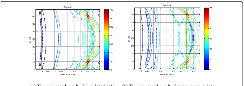
Figure 9, we can see that both the velocity and the cross-ing point are estimated correctly. The estimated velocity is 1.62 m/s, the crossing point is estimated at 10 and 40 m.

The simulated and experimental results show that the classical processing algorithm cannot obtain the correct the velocity estimation because of the mismatched target crossing position. Our new algorithm cannot only esti-mate the velocity, but also estiesti-mate the target crossing position correctly, although there is no range resolution in the baseline direction. In addition, the new algorithm extend the operation area, that is to say no matter where is the target crossing position, we can always obtain good estimations of thevanddT, contrary to the

classical processing algorithm only works in the

opera-tion area around dT/L = 0.5 (crossing near the

midpoint).

We should point out that there is an ambiguous crossing position in Figure 8. This is because the ence signal is symmetrical when the constructed refer-ence signal has the distance dTto the transmitter or to

the receiver. If we use the netted FSR, it is not difficult to solve the ambiguity problem of crossing position.

5. Conclusions

In this article, we have presented a signal processing method for the ground-based FSR system, including the target detection and the joint parameter estimation. It extended the operation area of the classical method.

The estimated parameters are very important for further requirements such as target classification and recogni-tion. The Crammer-Rao bounds for the accuracy of the estimations have also been given and be used to deter-mine the estimated step. The algorithm was tested both on simulated and experimental data, all of the results verify the effectiveness of our algorithm.

Acknowledgements

This study was supported by the National Natural Sciences Foundation of China (Grant Nos. 61172177, 61032009, 61120106004), and partially supported by the Electro-Magnetic Remote Sensing Defence Technology Centre, established by the UK Ministry of Defence, under Project No. 1-27.

Author details

1_{Department of Electronic Engineering, Beijing Institute of Technology,}

Beijing 100081, China2_{University of Birmingham, Edgbaston, B15 2TT, UK}

3_{School of Electronic Information, Soochow University, Suzhou, Jiangsu}

215021, China

Competing interests

The authors declare that they have no competing interests.

Received: 15 May 2011 Accepted: 11 April 2012 Published: 11 April 2012

References

1. RJ Boyle, Comparison of monostatic and bistatic bearing estimation

performance for low RCS targets. IEEE Trans AES.30(3), 962_–968 (1994)

2. NJ Willis,Bistatic Radar(Technology Service Corporation, Raleigh, 1995)

3. M Cherniakov (ed.),Bistatic Radar: Principles and Practice(Wiley & Sons, New

York, 2007)

4. V Chernyak,Fundamentals of Multisite Radar Systems(Gordon and Breach

Science Publishers, NV, 1998)

5. PY Ufimtsev, Comments on the diffraction principles and limitations of RCS

reduction techniques. Proc IEEE.84(12), 1830_–185 (1996)

6. MI Skolnik,Introduction to Radar Systems(McGraw-Hill Book Company, New

York, 1980), p. 558

7. VV Chapurskiy, VN Sablin, SISAR: shadow inverse synthetic aperture

radiolocation, inProc Int Radar Conf 2000, Washington, DC, USA, 332_–328

(2000)

8. AV Myakinkov, Optimal detection of high-velocity targets in forward

scattering radar, in5th International Conference on Antenna Theory and

Techniques, Kyiv, Ukraine, 2005, 345–347 (24–27 May2005)

(a) The processed result of simulated data (b) The processed result of experimented data

Velocity (m/s)

dT

(m

)

Contour

0.2 0.4 0.6 0.8 1 1.2 1.4 1.6 1.8 5

10 15 20 25 30 35 40

50 100 150 200 250 300 350 400

Velocity (m/s)

dT

(m

)

Contour

0.2 0.4 0.6 0.8 1 1.2 1.4 1.6 1.8 5

10 15 20 25 30 35 40

10 20 30 40 50 60 70

9. AB Blyakhman, AG Ryndyk, SB Sidorov, Forward scattering radar moving

object coordinate measurement, inThe Record of the IEEE 2000 International

Radar Conference, Alexandria, VA, 678–682 (7–12 May 2000)

10. DM Gould, RS Orton, RJE Pollard, Forward scatter radar detection, inRadar

2002, Edinburgh, UK, 36–40 (15–17 October 2002)

11. M Cherniakov, R Abdullah, P Jan_čovi_č, M Salous, V Chapursky, Automatic

ground target classification using FSR, inIEE Proceedings Radar, Sonar and

Navigation.153(5), 427_–437 (October 2006). doi:10.1049/ip-rsn:20050028

12. R Abdullah, M Cherniakov, P Jančovič, M Salous, Progress on using principle

component analysis in FSR for vehicle classification, inInt Workshop on

Intelligent Transportation - WIT, Hamburg, Germany, 7–12 (2005)

13. M Cherniakov, R Abdullah, V Chapursky, Short range forward scattering

radar, inInt Radar Conf, 322_–328 (October 2004)

14. R Abdullah, M Cherniakov, P Jančovič, Automatic vehicle classification in

forward scattering radar, in1st Int Workshop on Intelligent Transportation

-WIT, Hamburg, Germany, 7–12 (2004)

15. M Cherniakov, M Salous, M Kostylev, R Abdullah, Analysis of forward

scattering radar for ground target detection, in2nd European Radar Conf.,

Paris, France, 145–148 (2005)

16. M Cherniakov, M Salous, P Jančovič, R Abdullah, V Kostylev, Forward

scattering radar for ground targets detection and recognition, inDefence

Technology Conf, Edinburgh, UK, A-12 (2005)

17. V Sizov, M Cherniakov, M Antoniou, Forward scattering radar power budget

analysis for ground targets, inIEE Proc Radar sonar and Navigation.1(6),

437–446 (2007). doi:10.1049/iet-rsn:20060174

18. T Long, C Hu, M Cherniakov, Ground moving target signal model and

power calculation in forward scattering micro radar. Sci China Ser F Inf Sci.

52(9) (2009). doi:10.1007/s11432-009-0154-1

19. T Long, C Hu, T Zeng, XL Li, Physical modeling and spectrum spread

analysis of surface clutter in forward scattering radar. Sci China Inf Sci.53,

1–14 (2010). doi:10.1007/s11432-010-4085-7

20. C Hu, T Long, T Zeng, Statistic characteristic analysis of forward scattering

surface clutter in bistatic radar. Sci China Inf Sci.53, 1_–12 (2010).

doi:10.1007/s11432-010-4119-1

21. VI Kostylev, M Cherniakov, Analysis of the signal model for forward

scattering radar in case of a small target, inProceedings of the 5th European

Radar Conference, Munich, Germany, 126_–129 (2007)

22. H Cheng, M Antoniou, M Cherniakov, V Sizov, Quasi-optimal signal

processing in ground forward scattering radar, inRADAR‘08. IEEE, Radar

Conference, Roman, Italy, 1–6 (2008)

23. V Trees, L Harry,Detection, Estimation, and Modulation Theory, (John Wiley &

Sons, New York, 1971)

doi:10.1186/1687-6180-2012-80

Cite this article as:Zenget al.:Joint parameter estimation and

Cramer-Rao bound analysis in ground-based forward scatter radar.EURASIP

Journal on Advances in Signal Processing20122012:80.

Submit your manuscript to a

journal and benefi t from:

7Convenient online submission

7Rigorous peer review

7Immediate publication on acceptance

7Open access: articles freely available online

7High visibility within the fi eld

7Retaining the copyright to your article