Pole Assignment Using State Feedback with Time Delay in Friction Induced Vibration Problems
Abstract
Linear, friction-induced vibration and aeroelastic flutter problems are governed by second-order differential equations of motion in which the stiffness matrix and often damping matrix are asymmetric. Asymmetric systems are prone to unstable vibration (flutter) as a parameter reaches a critical value, when the real part of a pair of complex poles crosses the vertical imaginary axis of the s-plane from left to right. It is important and useful to shift the unstable poles to the left-hand half of the complex pole plane for stability. Pole assignment by means of active control introduces inherent time delays in the feedback control loop.
1. Introduction
Undesirable vibration may be reduced in a number of ways. One way is to shift the frequencies or poles of a structure or machine (referred to as a system in general) to some desirable values to avoid resonance. Another way is to assign zeros to certain locations of the system for some excitation frequencies so that vibration at those locations is absorbed for some known excitation frequencies. Pole and zero assignment by means of structural modifications as a way of passive vibration control has been widely studied and applied. One technique to assign frequencies is the rank-one modification put forward by Weissenburger [1] and extended by Pomazal and Synder [2].
Active vibration control to assign poles and zeros has also attracted attention in recent years. Traditionally vibration control problems are addressed in a state-space form leading to systems of first-order differential equations [3]. However, vibration control problems are naturally governed by second-order differential equations. Therefore devising control strategies in second order setting is computationally efficient and can lead to new findings [4]. Singh and Ram [5] established the conditions whereby the steady-state response of a damped symmetric system was absorbed by active control and demonstrated this with numerical examples. Chu [6] studied pole assignment to second-order symmetric and asymmetric systems. Datta and his colleagues [7] seemed to be the first researchers to make partial pole assignment to symmetric systems. They went further to make partial eigenstructure assignment [8] in which in addition to the eigenvalues the eigenvectors are also assigned to shape the desired response of the closed loop system. Qian and Xu [9] studied robust partial pole assignment. Recently, Pratt et al [10] considered the effect of time-delay in assigning poles to symmetric systems.
It is well known that the knowledge and accuracy of system matrices (mass, stiffness and sometimes damping matrices) are critical when assigning poles and zeros by active control, including those used in developing model based control [4-10]. Ram and Mottersehad [11] put forward a receptance-based inverse method for assigning poles and zeros to symmetric systems using state-feedback, which has distinct advantages over other methods for assigning poles and zeros. For example, the knowledge of mass, stiffness and damping matrices, though useful is not required in this method, so that modelling errors can be avoided. Ram et al. [12] also studied the effect of time-delay using the receptance method. Recently, the second author of this paper extended the receptance-based inverse method in order to control asymmetric systems [13]. A comprehensive review on the active vibration control method can be found in the review paper by Alkhatib and Golnaraghi [14].
2. Pole Assignment to Asymmetric Systems with Time Delay
The equations of motion of discretised linear vibration systems under conventional loads have symmetric mass, stiffness and damping matrices. However, when some internal forces such as friction and aerodynamic load are present, these system matrices can be asymmetric. Examples can be found in [15, 16]. In dynamics context, they are self-excited vibrations and susceptible to flutter instability. At high enough value of friction coefficient or air speed, the uncontrolled asymmetric system undergoes flutter instability. Therefore, for an asymmetric system, it is important to be able to assign negative real parts of the complex poles to stabilise an otherwise unstable system. This was the theme of a recently published work [Error: Reference source not found] by the first second author.
The linear equation of motion of a second-order damped dynamic system associated with friction induced vibration problem is represented as,
,
where , are structural symmetric matrices and the stiffness matrix is composed of symmetric structural stiffness and asymmetric stiffness matrix
of dimension , is controlling force and is external excitation. Note that the damping matrix can also be asymmetric [Error: Reference source not found] and be dealt with in the same way by the approach proposed here. The poles of a structure (a symmetric system) with non-negative viscous damping are complex with non-positive real parts. However, an asymmetric system with non-negative viscous damping can have complex poles with positive real parts or even positive real poles, indicating flutter instability or divergence.
In the absence of external force , and with the choice of controlling force the closed loop dynamics of the system associated with is ,
,
where, is the control location vector and the scalar controlling force has the following form
,
with and to bebeing proportional acceleration, velocity and displacement feedback control gains. The dynamics of the uncontrolled system with can be expressed in s-domain as
where, s is a complex variable and q(s) and p(s) are the Laplace transforms of the displacement and force vectors respectively. Similarly, when a single active control force in is considered the closed loop system dynamics in Laplace domain becomes
With state-feedback control form as introduced in [Error: Reference source not found] the closed-loop system becomes
.
It was shown [Error: Reference source not found] that active damping and active mass together or active damping and active stiffness together was capable of assigning all desired complex poles using the receptances of a small number of degrees-of-freedom of the symmetric part of the whole system, regardless of the location and number of the actuators.
Real control always involves time delay. It is inherent of a system, as it takes time to measure data and process them, compute the control force, transmit data and signals and finally apply the control force to the system [Error: Reference source not found]. Time delay is usually detrimental to the performance of the closed-loop system. Fuller et al. [17] showed that a small time delay could reduce the effective damping and thus destabilise a system. Ram et al. [Error: Reference source not found] separated the poles of closed-loop system into two sets: the primary set consists of the 2n poles of the system that control the dynamics of the system and the secondary set consists of the other (infinite number of) poles due to the delay. They demonstrated the necessity of a posterior analysis to ascertain that the poles of the system with delay do not have positive real parts. Singh et al. [18] studied zero assignment to systems with time delay. It should be pointed out that in all the published works on pole assignment the open-loop second-order systems with time delay are symmetric. This paper studies pole assignment to asymmetric open-loop second-order systems with time delay. Time delay can be intentionally introduced to help reduce vibration and increase stability [19].
By introducing the time delay in the feedback control force such that
,
where , and are constant time delays associated with the acceleration, velocity and displacement state feedback respectively, the closed loop system has the following form in Laplace domain,
When a time delay is small, then equation would lead to a polynomial eigenvalue problem which has a finite number of poles (eigenvlaues). For example, the second-order Taylor expansion of
The receptance matrix of the symmetric part of the open-loop system is
,
which are generally obtained by the sensor and actuators and by extracting the frequency response function. Similarly, the receptance matrix of the symmetric part of the closed-loop system is
From the Sherman-Morrison formula, a closed-form expression of can be found as
.
Multiplying both sides of equation with yields
.
The poles of the closed-loop system with time delay must make
.
If all the poles of the time-delay system have negative real parts, then the system is stable [Error: Reference source not found].
3. Application and numerical example
To demonstrate how the method is used, a simulated numerical example studied in [Error: Reference source not found] is used here. The system is shown in Figure 1 below.
Figure 1. An asymmetric system of friction-induced vibration
The system has three masses with having a degree-of-freedom in the x (horizontal) direction, having a degree-of-freedom in the y (vertical) direction, and having degrees-of-freedom in both directions. The belt moves at a constant speed. and are respectively the friction force and (pre-compression) normal force acting at the slider-belt interface. The sliding friction at the slider-belt interface is governed by Coulomb friction whose static and kinetic friction coefficients are taken to be the same. This is a simplification and avoids stick-slip vibration. M, C and K, and E corresponding to displacement vector are respectively
, ,
,
Using the bisection method and MATLAB polyeig function, the critical point of the open-loop system is found to be , where the system becomes unstable (flutter instability). The proposed method is used below to assign poles to the systems at various frictional coefficient values .
For this particular example, equation (10) becomes
where are all the elements in the third column of the closed-loop receptance matrix . The complex poles s of the asymmetric system must satisfy the equation below
1 J.T. Weissenburger, Effect of local modifications on the vibration characteristics of linear systems, Transactions of ASME, Journal of Applied Mechanics, Vol. 90, (1968), pp. 327–33. 2 R.J. Pomazal, V.W. Snyder, Local modifications of damped linear systems, AIAA
Journal, Vol. 9, (1971), pp. 2216–2221.
3 T. T. Soong, Active Structural Control: Theory and Practice, Longman Scientific & Technical, Harlow, England (1990).
4 D.J. Inman, Active modal control for smart structures, Philosophical Transactions of the Royal Society of London A,Vol. 359, (2001), pp. 205-219.
5 K. V. Singh, Y. Ram, Dynamic absorption by passive and active control, ASME Journal of Vibration and Acoustics, Vol. 122, No. 5, (2000), pp. 429–433.
6 E. K. Chu, Pole assignment for second-order systems, Mechanical Systems and Signal Processing, Vol. 16, (2002), pp. 39-59.
7 B. N. Datta, S. Elhay, Y. M. Ram, Orthogonality and partial pole assignment for the symmetric definite quadratic pencil, Linear Algebra and Applications, Vol. 257, (1997), pp. 29-48.
8 B. N. Datta, S. A. S. Elhay, Y. M. Ram, D. R. Sarkissian, Partial eigenstructure assignment for the quadratic pencil, Journal of Sound and Vibration, Vol. 230, (2000), pp. 101-110.
9 J. Qian, S. F. Xu, Robust partial eigenvalue assignment problem for the second-order system, Journal of Sound and Vibration, Vol. 282, (2005), pp. 937-948.
10 J. M. Pratt, K. V. Singh, B. N. Datta, Quadratic partial eigenvalue assignment problem with time delay for active vibration control, Journal of Physics: Conference Series, Vol. 181, Article No. 012092, (2009).
11 Y.M. Ram, J.E. Mottershead, Receptance method in active vibration control, American Institute of Aeronautics and Astronautics Journal, Vol. 45, (2007), pp. 562-567.
12 Y. M. Ram, A. Singh, J. E. Mottershead, State feedback control with time delay, Mechanical Systems and Signal Processing, Vol. 23, (2009), pp. 1940–1945.
13 H. Ouyang, Pole assignment of friction-induced vibration for stabilisation through state-feedback control, Journal of Sound and Vibration, Vol. 329, (2010), pp. 1985–1991.
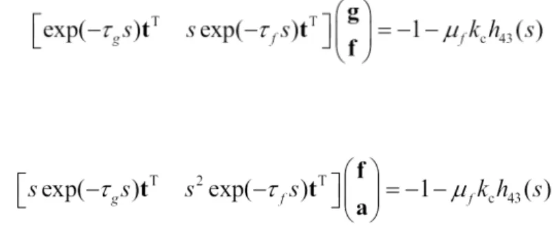
Substituting equation into and further manipulation of the resultant equation yields
For active damping and active stiffness together and active damping and active mass together, equation becomes respectively
and
It was found [Error: Reference source not found] that the open-loop system without time delay became unstable when =0.3868 and the four complex conjugate pairs of poles at this critical point are
,
where . It was also found [Error: Reference source not found] that active damping and active stiffness together or active damping and active mass together was capable of assigning poles with negative real parts to the open-loop system to stabilise it. It will be found whether poles with negative real parts may be assigned when there is time delay and further whether introducing time-delay will alleviate the control effort. Suppose the open loop poles in are shifted to desired closed loop poles values
.
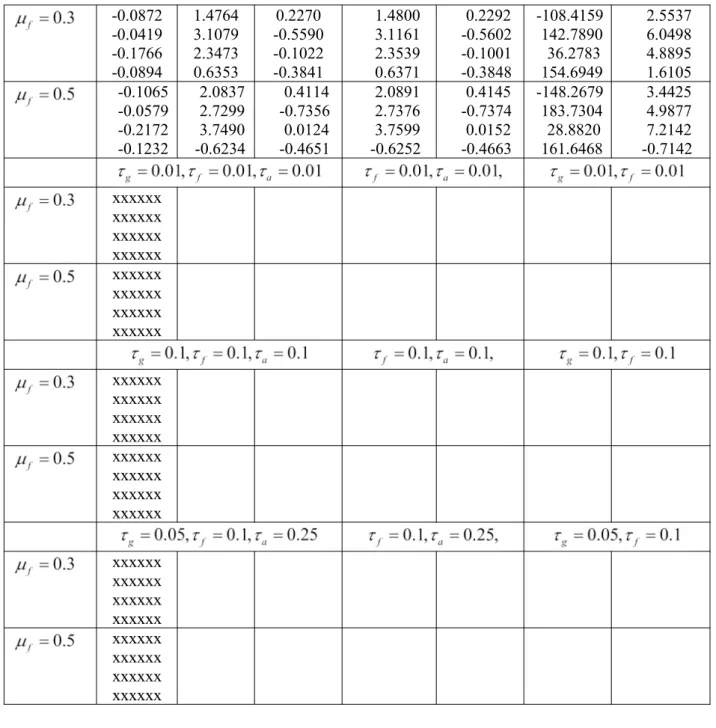
For such pole placement control gains associated with the active acceleration, damping and stiffness, with control distribution vector , are obtained at various delay times are given in Table 1.
Table 1. Control gains at various delay times for placing to new value
I am planning to have the table with control gains for different cases. I will fill the table if you think it is appropriate and I have the codes ready
Active acceleration, velocity and displacement feedback
Active acceleration and velocity feedback
-0.0872 -0.0419 -0.1766 -0.0894 1.4764 3.1079 2.3473 0.6353 0.2270 -0.5590 -0.1022 -0.3841 1.4800 3.1161 2.3539 0.6371 0.2292 -0.5602 -0.1001 -0.3848 -108.4159 142.7890 36.2783 154.6949 2.5537 6.0498 4.8895 1.6105 -0.1065 -0.0579 -0.2172 -0.1232 2.0837 2.7299 3.7490 -0.6234 0.4114 -0.7356 0.0124 -0.4651 2.0891 2.7376 3.7599 -0.6252 0.4145 -0.7374 0.0152 -0.4663 -148.2679 183.7304 28.8820 161.6468 3.4425 4.9877 7.2142 -0.7142 xxxxxx xxxxxx xxxxxx xxxxxx xxxxxx xxxxxx xxxxxx xxxxxx xxxxxx xxxxxx xxxxxx xxxxxx xxxxxx xxxxxx xxxxxx xxxxxx xxxxxx xxxxxx xxxxxx xxxxxx xxxxxx xxxxxx xxxxxx xxxxxx
Table 1. Active damping and stiffness vectors to assign poles with
-1 9i, -1 13.5i, -1 18i, -1 22i at various delay times and the amount of energy consumed Delay times Active damping vector f Active stiffness vector g Energy
0.0793 0.0753 0.0668 0.0678 0.0643
which is for time-delay systems
should be computed, where T is a long-enough time interval that should cover several longest periods of the vibration concerned. A Matlab code is programmed to compute the response of the time-delay closed-loop system in the time-domain governed by equation
and then the energy involved defined by equation (1823). The results are given in the last column of Table 1 in the case of initial conditions of:
and zero initial velocities. Please note that in equations -, u, x and p are respectively the control force, physical displacement and force vectors (functions of time), and should not be confused with the same symbols (their Laplace transforms) in the rest of the paper.
To validate whether the gains shown in Table 1 are correct, the desired poles are substituted back into equation and indeed the resultant determinant of the coefficient matrix is very close to zero, indicating indeed the desired poles are successfully assigned. When the gains given in Table 1 are substituted back into equation , the poles obtained by solving equation are listed in Table 2.
It can be seen that the second-order Taylor expansion of the complete equation leads to poles that are very close to the desired values when delay times are very small (see the third and fourth rows), but are noticeably different for higher poles when delay times are big (the last row). So it is expected higher-order Taylor expansion would give more accurate results when delay times are big.
Table 2. Poles actually realised at various delay times when using the second-order Taylor expansion, equation
Delay times Poles actually realized
-1.00 9.00 i, -1.00 13.5 i, -1.00 18.0 i, -1.00 22.0 i -1.00 9.00 i, -1.00 13.5 i, -1.00 18.0 i, -1.00 22.0 i
-1.00 9.00 i, -1.00 13.5 i, -1.00 18.0 i, -1.00 22.0 i -1.00 9.00 i, -1.00 13.5 i, -0.99 18.0 i, -0.98 22.1 i -1.00 9.01 i, -0.97 13.6 i, -0.91 18.1 i, -0.50 23.1 i
4. Stability of the Time Delayed System
control gains with and equal time delay in feedback loop ,
where, such that with a infinite number of roots or poles . In general, the characteristic quadratic pencil associated with the controlled system without time delay in the feedback loop is a polynomial. Hence for the n dimensional system it will have 2n roots. The location of these roots in the complex plane defines the stability of the system. The system having eigenvalues with real positive part is considered to be unstable
and those having eigenvalues with negative real parts or purely imaginary are considered to be stable and neutral respectively. However the characteristic equation of a controlled system with delay is a quasi-polynomial or transcendental functions and has an infinite number of roots in the complex plane , which satisfies the associated transcendental eigenvalue problem (TEP) [Error: Reference source not found] in the following form,
.
Hence by assigning the 2n open loop poles with negative real part may not necessarily make the system stable because there may be one or more unstable roots satisfying the eigenvalue problem . One way to perform the stability analysis is to compute the roots associated with the TEP . Because, there are infinite eigenvalues in the complex plane, the primary eigenvalues (those closer to imaginary axis) may be computed or needs to be approximated for posteriori stability analysis [Error: Reference source not found]. For example, the true eigenvalues satisfying can be computed by Newton’s Eigenvalue Iteration Method as shown in [20], in which by defining,
,
the TEP may be solved numerically by choosing an initial guess for and by finding the smallest eigenvalue, of the following generalized eigenvalue problem,
.
The improved estimate for the next iteration is obtained by substituting , for , where is the number of iterations when is sufficiently small. This process can be repeated for any desired number of eigenvalues computed for stability tests.
,
For example by following [Error: Reference source not found], the approximated system matrices obtained by Taylor series expansion are:
,
with . For a given domain in a complex plane,
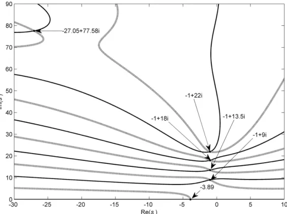
the eigenvalues of can also be graphically represented by the root-finding algorithm given in [21,22].
Figure 2. The roots in the complex plane of the controlled system. Solid line contours: Dotted line contours:
It is important to note that the root finding algorithm by [Error: Reference source not found] and is capable of computing the eigenvalues in any defined complex domain whereas the Taylor series approximation estimates the finite number of eigenvalues and they are accurate only for very small time delay , as described in [23]. Hence for larger time delay, in our case they may produce incorrect closed loop unstable eigenvalues as shown in Table 3, for eigenvalues obtained from the second- order Taylor Series approximation.
Table 3: The closed loop eigenvalues obtained by different techniques Quasi
polynomial TEP Taylor Series(First Order) (Second Order)Taylor Series
, and
-1 9i -1 13.5i
-1 18i
-1 9i -1 13.5i
-1 18i
-1.0019 9.0008i -1.0064 13.5049i
-1.0081 18.0127i
-1 22i -1 22i -1.0667 22.0454i -0.9969 22.0050i -2371.8
, and
-1 9i -1 13.5i
-1 18i -1 22i -27.05 77.58i
-3.89
-1 9i, -1 13.5i -1 18i, -1 22i -27.05 77.58i
-3.89
-33.67 140.62i -37.56 203.55i -40.33 266.45i -42.48 329.34i
-1.0851 9.4048i -0.9723 14.4210i
-0.6691 18.8045i -5.2677 -22.1874 -0.9253 9.0852i -0.7418 13.7895i -0.6206 18.3667i 5.0313 28.2684i -3.9877
Now instead of computing the closed loop eigenvalues, as demonstrated by several approaches discussed earlier in this section, the stability analysis of time-delay systems can be performed by well-established methods either in frequency-domain and/or in time-domain analysis [Error: Reference source not found],[24-25] . In the remaining section frequency domain analysis described in Gu et. al. [Error: Reference source not found] is formulated and stability tests were conducted while computing the critical time delay required for stability of closed loop system. The closed loop dynamics of the time delayed system,
,
with the choice of the controlling force,
,
can be written as,
.
The controlled system with single time delay , can be expressed in the following state-space form, given in [Error: Reference source not found],
where, is the system state and
.
supplementary sufficient condition for delay independent stability is given by
where denotes the spectral radius: , the maximum absolute value of the eigenvalues.
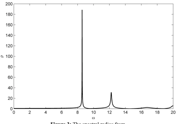
The above tests are to check if the system is delay independent stable, . however However, for some values of the delay, the system can have positive eigenvalues and such systems are termed as delay-dependent stable [Error: Reference source not found]. In such cases, the “delay-margin” and “critical time delay” of the system can be estimated by stability analysis. For example, when the lower bound of the interval of delay is 0, the upper bound of the interval defining the delay margin can be computed. It is also possible to find systems for which the lower bound of the interval is non-zero and the system is not stable for = 0. It is shown in Gu et al. [Error: Reference source not found] and Gouaisbaut and Peaucelle [26] that the stability margin for a time delayed system can be computed and it can be shown that the system may be stable for all constant delay in a given interval. Frequency-sweeping tests are shown in [Error: Reference source not found] to find the critical delay values at which the characteristic roots intersect the stability boundary, i.e. the imaginary axis, thus rendering the system unstable. It is shown that in addition to criteria , if the system is stable at with then by computing the quantity
the critical time delay can be obtained. Hence the system is stable for all , but becomes unstable at .
Figure 3: The spectral radius from
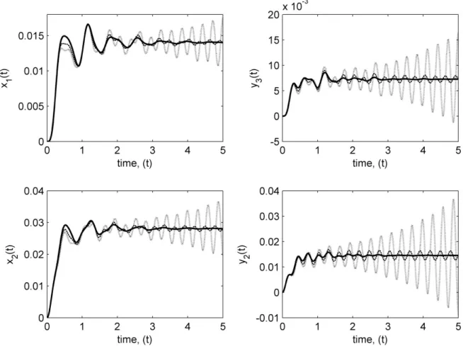
Figure 4: The step response of the controlled system (Solid line: , Dashed line: and Dotted line: )
5. Conclusions
This paper studies the assignment of complex poles to asymmetric second-order dynamic systems using state feedback control of active damping and active stiffness, with time delays either inherent in the systems or introduced intentionally. The inverse method is based on receptances of the symmetric part of the open-loop system, which can be directly measured to avoid modelling errors. It is found from a simple simulated example of a four-degree-of-freedom friction-induced vibration problem that active damping and active stiffness together is capable of precisely assigning n pairs of complex poles with negative real parts to asymmetric systems. As delay times increase, the gains required to assign desired poles become increasingly different from the gains when there is no time delay and the energy required by the actuators in general decreases moderately. This indicates that deliberate introduction of time delay may reduce cost of stabilising an unstable asymmetric system by actuators.
Time-delay systems have infinite number of poles. Those unassigned poles could have positive real parts. In that case, the system is not yet fully stabilised, unlike a delay-free system. How to guarantee that the time-delay systems are stabilised by assigning only n pairs of poles remains an issue and is being studied by the authorsin the paper. A formula for estimating stability margin for time delay is described and presented with a numerical example.
Finally a multi-input control force of state-feedback, or output-feedback can also be used to assign n pairs of complex poles with negative real parts to asymmetric systems.
Acknowledgements
The first author would like to acknowledge the Royal Academy of Engineering/Leverhulme Trust Senior Fellowship for supporting the research reported in this paper. The second first author’s research is supported in part by the Philip and Elaina Hampton Fund for Faculty International Initiatives at Miami University, 2009-10.
References
15 G. Sheng, Friction-induced Vibration and Sound: Principles and Applications, CRC Pr I Llc (2007)
16 J. R. Wright, J. E. Cooper, Introduction to Aircraft Aeroelasticity and Loads, John Wiley & Sons (2007).
17 C.R. Fuller, S.J. Elliott, P.A. Nelson, Active Control of Vibration, Academic Press (1996), New York
18 K.V Singh, B.N. Datta, M. Tyagi, Closed form control gains for zero assignment in the time-delayed system. ASME Conference Paper No. DETC2007-34819, to appear in ASME Journal of Computational and Nonlinear Dynamics, (2010)
19 K. Gu, V.L. Kharitonov, J. Chen, Stability of Time-Delay Systems, Birkhauser (2003). 20 Singh K. V. and Ram Y. M., “Transcendental eigenvalue problem and its applications”,
AIAA Journal, Vol. 40 (7), pp.1402-1407, 2002.
21 Vyhlidal, T. and Zitek, P., “Quasipolynomial mapping based rootfinder for analysis of time delay systems”, Time Delay Systems 2003 - A Proceedings volume from the 4th IFAC workshop, Rocquencourt, France, Elsevier: Oxford, pp. 227-232, 2003.
22 Vyhlidal T., P. Zitek, “Mapping based algorithm for large-scale computation of quasi-polynomial zeros”, IEEE Transactions on Automatic Control, Vol. 54 (1), pp. 171-177, 2009. 23 Hu H.Y. and Wang, Z.H., Dynamics of controlled mechanical systems with delayed
feedback, Springer, New York, 2002.
24 Stepan G., Retarded dynamical systems: stability and characteristic functions, Essex Longman Scientific and Technical, 1989.
25 S.-I. Niculescu. Delay effects on stability. A robust control approach, volume 269. Springer-Verlag:Heidelbeg, 2001.